Loading a Program into Ghidra

Before you get started, you need to load a program. This is not as straightforward a task as you might think. It’s not as simple as just clicking on File/Open and pointing it at the program you want to look at. Ghidra is project-oriented. You can work collaboratively in Ghidra or work alone. Ghidra refers to this as a shared or non-shared project. So, we need to start with creating a project before we can get to the fun part of looking at a program.

Creating a Project

To create a new project, Choose File → New Project and click through the wizard to choose your project directory. You will also be asked if you want your project to be Shared or Non-Shared. A Shared project can be viewed and analyzed by multiple parties, and requires a running Ghidra server. For simply exploring the Ghidra interface the first time, choose Non-Shared.

Give your project a name, click Finish, and your project should now appear in the main Ghidra window under Active Projects.

Once you have created your project, you can now load binaries in for analysis. To do this, click File → Import File and choose the file you wish to analyze. Choose Select File to Analyze and choose the options on the next pop-up window, pertaining to the format and filetype. You can also import files simply by dragging them into the Ghidra window.

Next you will be presented with a dialog box about the file to be imported, seen in Figure 3-1. Ghidra will try to auto-detect the format of the binary, such as if it is an ELF or PE file, as well as important information such as the compiler used to compile the binary. You may change these options if Ghidra has incorrectly detected a format.

Figure 3-1. Importing a file

Once the file has been imported, you should get a window labeled Import Results Summary. This will display details of the file as it was imported, and confirm that your file has been loaded into Ghidra successfully. Here you can see details such as number of funtions detected, number of memory blocks, Endian-ness, required libraries, and other information. In the Additional Information box below the summary you will also see any errors that occurred, or missing data about the binary. The summary is shown in Figure 3-2.

Figure 3-2. Importing results

Your file should now appear under your project in the Active Project: <Project Name> window. You are now ready to analyze the file using your toolset.

Overview of the Interface

Within the Project Manager window and the toolbar, there is the Tool Chest. This is where your tools will appear as you add new plug-ins. At first install you should see two tools: CodeBrowser (shown as a green dragon icon) and Version Tracking (shown as an icon of two footsteps). These are seen in Figures 3-3 and 3-4.

Figure 3-3. CodeBrowser icon

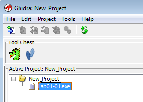
Figure 3-4. Version Tracking icon

You will likely want to begin examining the file using CodeBrowser.

Using CodeBrowser

To analyze your file with a given tool, click and drag the file over the tool you wish to use. For this first overview, drag it over the CodeBrowser (green dragon) icon. This should open the file in CodeBrowser.

You will then be asked, “<Filename> has not yet been analyzed. Would you like to analyze it now?” Click yes to start the auto-analysis process. The next window will present you with several auto-analysis options, many of them already checked, shown in Figure 3-5.

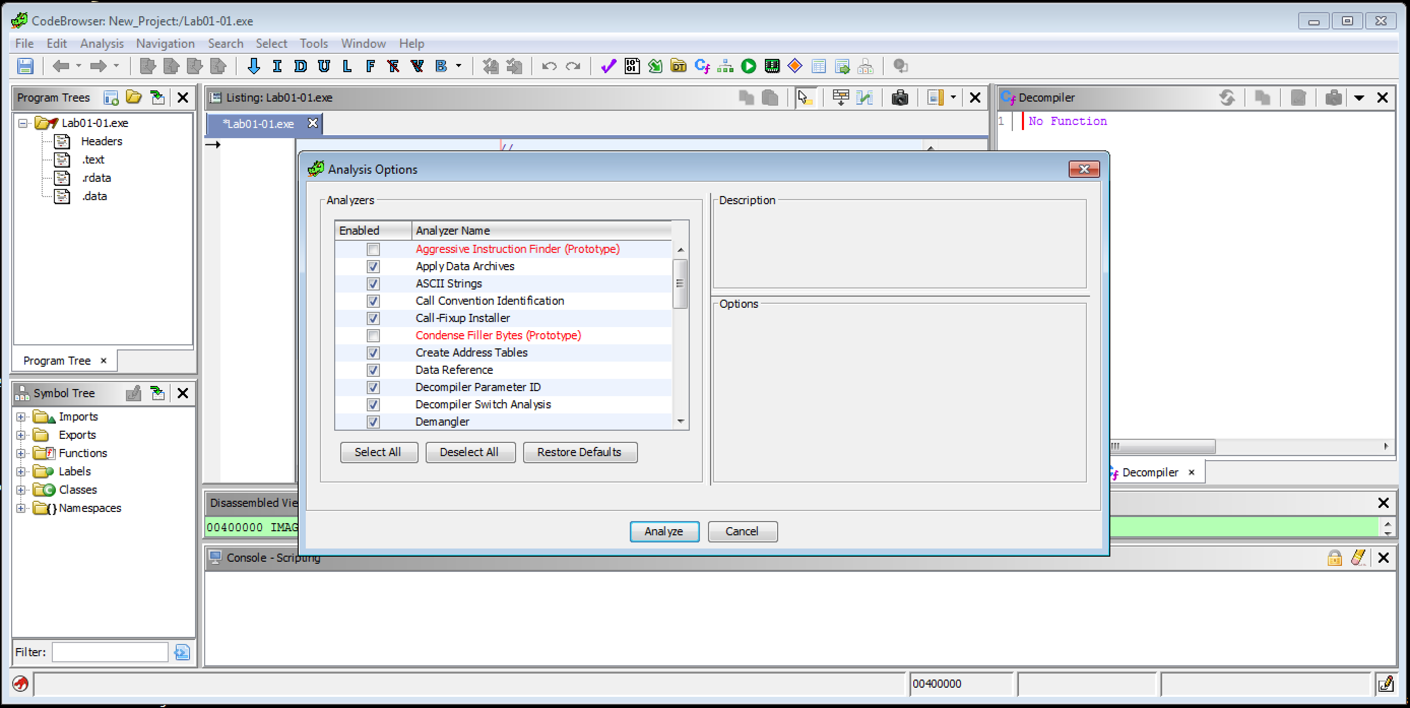
Figure 3-5. Analysis options

The CodeBrowser project window is modular with many different options. The various windows you can utilize are listed under “Windows.” The default view will contain the following windows:

• Program Trees

• Symbol Tree

• Listing (Disassembly)

• Decompile

You can add windows by selecting them in the Windows drop-down. You may also move windows by clicking and dragging them to different locations in the interface.

Disassembling a Program

The file you loaded will be disassembled as soon as you open a project in the CodeBrowser. Once you open a program, the first and most obvious thing you will see is all of the assembly language right in the middle of the CodeBrowser application. So, there is nothing really to do there. However, that does not mean that working with the code and understanding what you are looking at is nearly as straightforward.

The Disassembly view of the program will appear in the Listing window. You can simultaneously view the disassembly and the decompiled view, and as you traverse the disassembly, the decompiled view of that code will appear as well. You will only get decompilations if you have moved into a function. Otherwise, you get a note indicating that you are not in a function. Where you do get a decompilation, you can see exactly what part of the decompiled code is represented by the disassembly. In Figure 3-6, the assembly language MOVSXD RDX,EAX aligns with the line in the source code starting if (*(int *)). If you are less fluent in assembly language, this is very beneficial.

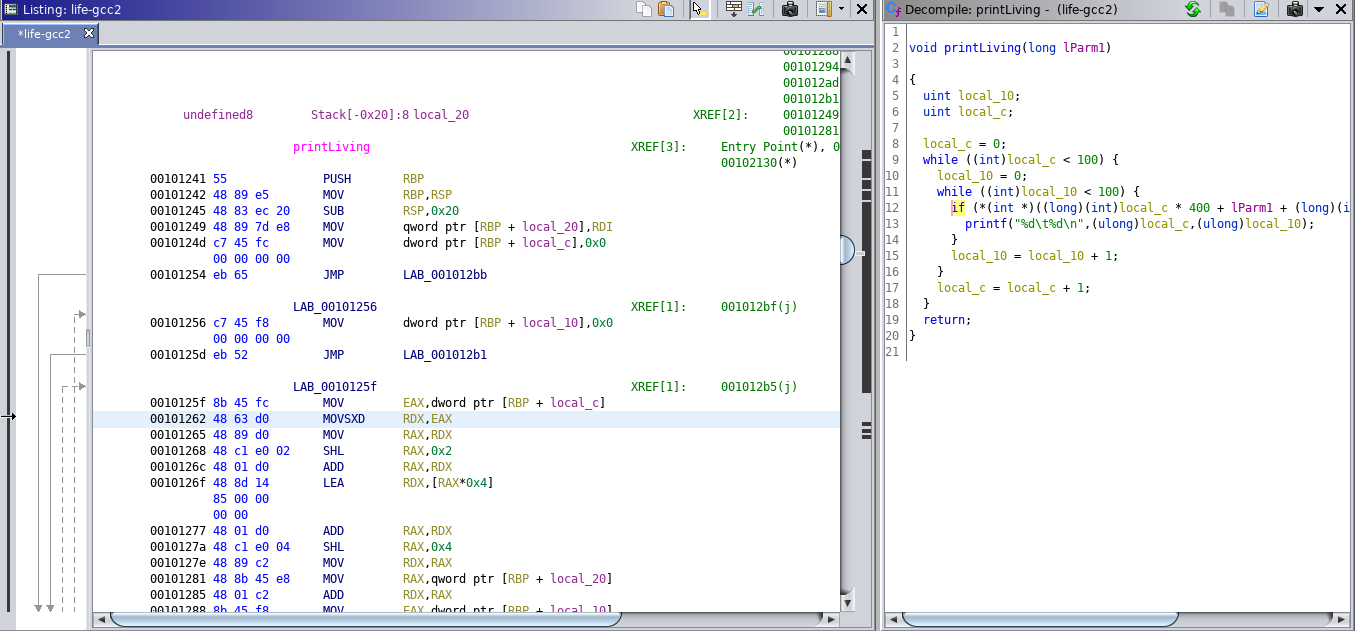
Figure 3-6. Correlating assembly and source code

On the lefthand side of the CodeBrowser application window, you will see some information that was provided by the metadata in the program. The particular code we’ve been looking at is an Executable and Linkable Format (ELF), used by Linux as the container that binaries and libraries are put into. If you look at the lefthand side of the CodeBrowser window, you can see the Program Tree window. This provides shortcuts to places in the disassembled code. As an example, the top listing in Figure 3-7 is .bss. This is shorthand for Block Started by Symbol and refers to the location where statically allocated variables are located. These are essentially variables that are known about and allocated at runtime. C compilers will carve out space for these variables but set them to 0 at compile time.

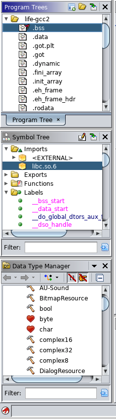
Figure 3-7. Program and Symbol Trees

Underneath the Program Trees is the Symbol Tree. A symbol is a named reference to a part of the program. These references may be useful if the program is allowing another executable access to code to run inside another process context. The external program has to call the specific resource by name, so there are labels assigned to these resources. The Symbol Tree is a list of all of these different resources. From here, you can not only see any symbol that has been marked as exported, meaning other programs can see the function from the outside, but also all imports.

The imports are important because they reveal outside sources of programmatic help. When a program uses external libraries, those libraries have exports that have names. Typically, the names are reflective of what the function or method does. With these names, we can see behaviors of the program without actually running the program. This doesn’t mean we know exactly how the program functions just because we have some function names. It does give hints as to functionality though. In Figure 3-2, for instance, you can see that the standard C library has been pulled into the program.

Graphing a Program

When analyzing malware, analysts often like to see how the functions within the program interact. Rather than trying to scroll back and forth between references, you can use the Function Graph option in Ghidra. This view will show you how various parts of the binary are linked. You can see the Function Graph for the executable we have been working with in Figure 3-8. This is just a partial Function Graph. The Graph view allows you to jump into each function separately.

Once you have the binary loaded into CodeBrowser, you can choose the Function Graph view by going to the toolbar and choosing Window → Function Graph. Keep in mind this will display a Function Graph for whatever function you have selected in the disassembly view.

Figure 3-8. Function Graph of a portion of the program

For our example binary, if you go to the Symbol Tree and open Functions, you will see “entry” at the bottom. While the entry point is not always the location of the main() function, in this case if you double-click “entry,” you will be taken to the location of the main() function. While this is selected, choose the Function Graph window and you will see the function laid out in a graph view. If you start with the main() function, you will get the disassembly of that function. If you want to trace the graph, you can follow each call statement into the function that is being called.

From this view you can see the main() function making two function calls to _populateGrid and _printGrid. To see these function calls more explicitly, you can also go to Window → Function Call Graph. This will display an abstracted view of all the calls made from one function to another. In this case you can drill down into _populateGrid and _printGrid to see _rand and _printf called, respectively. This allows you to quickly determine the end functionality of parent functions within the program. There is a third call to ___stack_chk_fail, which is a check to prevent buffer overflow and an artifact of compilation.

Further Analysis

The more you work with Ghidra, the more you will see the power that the platform has. The visual perspective on the program analysis, allowing you to follow the program from function call to function call in visual isolation using the Function Graph, is very powerful. If you are working with malware, you don’t want to try executing the program, which is what a debugger would be doing for you—allowing you to trace a program step by step. It gives you the ability to follow the entire execution path from one operation to the next. That’s not always useful. Having a way to visually inspect the program and easily follow the path of execution makes life much easier.

One aspect of a running program you may not take into consideration is the permissions assigned to different memory segments. This is especially important when it comes to analyzing malware or looking through a potentially vulnerable program. In Figure 3-9, you can see a memory map of our program. What you’ll notice is three columns marked R, W and X. These are the permissions on the memory segments. If you are not familiar with R, W, and X, they stand for Read, Write, and eXecute. You’ll see there are only a handful of segments that are marked X. These permissions on different segments help protect the memory space and, by extension, the program.

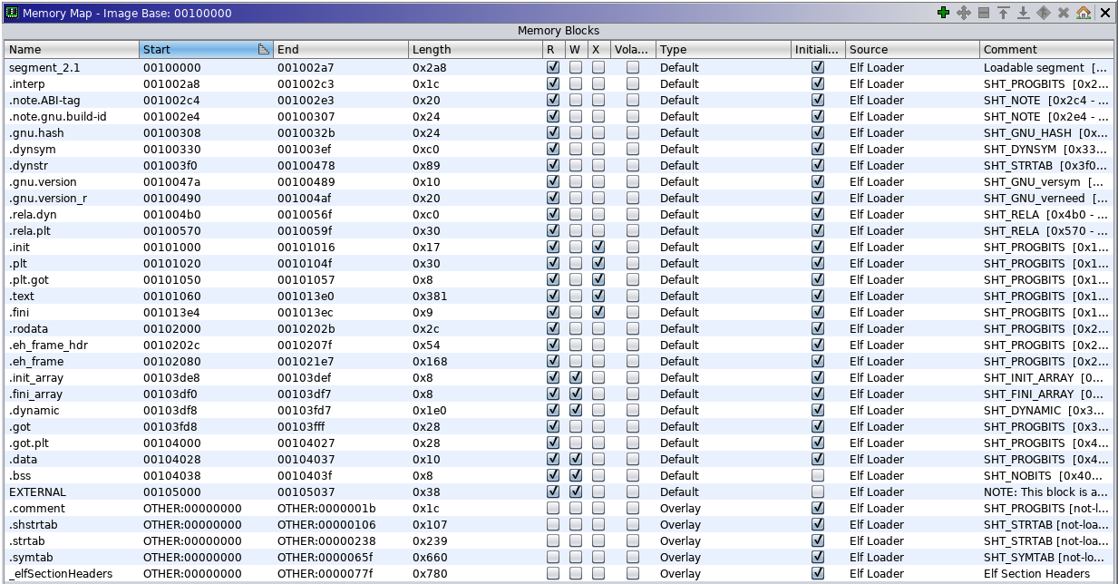
Figure 3-9. Memory map of the program

Segments where only data should be residing, like the stack for instance, should not have an execute permission set. With the execute permission set on the stack, buffer overflows within the process space can happen. Without the execute permission set, the attacker has to find other pathways to get their code executed. This may include a strategy like return to libc, where the attacker takes advantage of a known location of a shared library to get the program to do what the attacker wants it to do.

Of course, these are just an introductory set of capabilities for Ghidra. As you continue to work with it and investigate some, you will start to recognize how much power a tool like this has, especially for people who are trying to learn how programs work and how to get started with reverse engineering.