
Chapter 8. Motion
Like a flip book, animation on screen is created by drawing an image, then drawing a slightly different image, then another, and so on. The illusion of fluid motion is created by persistence of vision. When a set of similar images is presented at a fast enough rate, our brains translate these images into motion.
Frames
To create smooth motion, Processing tries to run the code inside draw() at 60 frames each second. A frame is one trip through the draw() and the frame rate is how many frames are drawn each second. Therefore, a program that draws 60 frames each second means the program runs the entire code inside draw() 60 times each second.
Example 8-2: Set the Frame Rate
The frameRate() function changes the speed at which the program runs. To see the result, uncomment different versions of frameRate() in this example:
defsetup():frameRate(30)# Thirty frames each second#frameRate(12) # Twelve frames each second#frameRate(2) # Two frames each second#frameRate(0.5) # One frame every two secondsdefdraw():frameRate
Note
Processing tries to run the code at 60 frames each second, but if it takes longer than 1/60th of a second to run the draw() method, then the frame rate will decrease. The frameRate() function specifies only the maximum frame rate, and the actual frame rate for any program depends on the computer that is running the code.
Speed and Direction
To create fluid motion examples, we use a data type called float. This type of variable stores numbers with decimal places, which provide more resolution for working with motion. For instance, when using ints, the slowest you can move each frame is one pixel at a time (1, 2, 3, 4, . . .), but with floats, you can move as slowly as you want (1.01, 1.01, 1.02, 1.03, . . .).
The data type of a variable depends on the value that you assign to it. To create a value of type float, include a decimal point as part of the number in your code. If you don’t include a decimal point, Python will create a value of type int. In the following code snippet, for example, the data type of variable var1 is float, whereas the data type of variable var2 is int:
var1=12.5# floatvar2=4# int
In Python, you can write arithmetic expressions that mix ints and floats (e.g., 6 * 0.5). The data type that results from such expressions is always float.
Example 8-3: Move a Shape
The following example moves a shape from left to right by updating the x variable:

radius=40.0x=-radiusspeed=0.5defsetup():size(240,120)ellipseMode(RADIUS)defdraw():globalxbackground(0)x+=speed# Increase the value of xarc(x,60,radius,radius,0.52,5.76)
When you run this code, you’ll notice the shape moves off the right of the screen when the value of the x variable is greater than the width of the window. The value of x continues to increase, but the shape is no longer visible.
Example 8-4: Wrap Around
There are many alternatives to this behavior, which you can choose from according to your preference. First, we’ll extend the code to show how to move the shape back to the left edge of the screen after it disappears off the right. In this case, picture the screen as a flattened cylinder, with the shape moving around the outside to return to its starting point:

radius=40.0x=-radiusspeed=0.5defsetup():size(240,120)ellipseMode(RADIUS)defdraw():globalxbackground(0)x+=speed# Increase the value of xifx>width+radius:# If the shape is off screen,x=-radius# move to the left edgearc(x,60,radius,radius,0.52,5.76)
On each trip through draw(), the code tests to see if the value of x has increased beyond the width of the screen (plus the radius of the shape). If it has, we set the value of x to a negative value, so that as it continues to increase, it will enter the screen from the left. See Figure 8-1 for a diagram of how it works.

Figure 8-1. Testing for the edges of the window
Example 8-5: Bounce Off the Wall
In this example, we’ll extend Example 8-3 to have the shape change directions when it hits an edge, instead of wrapping around to the left. To make this happen, we add a new variable to store the direction of the shape. A direction value of 1 moves the shape to the right, and a value of −1 moves the shape to the left:

radius=40.0x=110.0speed=0.5direction=1defsetup():size(240,120)ellipseMode(RADIUS)defdraw():globalx,directionbackground(0)x+=speed*directionifx>width-radiusorx<radius:direction=-direction# Flip directionifdirection==1:arc(x,60,radius,radius,0.52,5.76)# Face rightelse:arc(x,60,radius,radius,3.67,8.9)# Face left
When the shape reaches an edge, this code flips the shape’s direction by changing the sign of the direction variable. For example, if the direction variable is positive when the shape reaches an edge, the code flips it to negative.
Tweening
Sometimes you want to animate a shape to go from one point on screen to another. With a few lines of code, you can set up the start position and the stop position, then calculate the in-between (tween) positions at each frame.
Example 8-6: Calculate Tween Positions
To make this example code modular, we’ve created a group of variables at the top. Run the code a few times and change the values to see how this code can move a shape from any location to any other at a range of speeds. Change the step variable to alter the speed:

startX=20.0# Initial x coordinatestopX=160.0# Final x coordinatestartY=30.0# Initial y coordinatestopY=80.0# Final y coordinatex=startX# Current x coordinatey=startY# Current y coordinatestep=0.005# Size of each step (0.0 to 1.0)pct=0.0# Percentage traveled (0.0 to 1.0)defsetup():size(240,120)defdraw():globalx,y,pctbackground(0)ifpct<1.0:x=startX+((stopX-startX)*pct)y=startY+((stopY-startY)*pct)pct+=stepellipse(x,y,20,20)
Random
Unlike the smooth, linear motion common to computer graphics, motion in the physical world is usually idiosyncratic. For instance, think of a leaf floating to the ground, or an ant crawling over rough terrain. We can simulate the unpredictable qualities of the world by generating random numbers. The random() function calculates these values; we can set a range to tune the amount of disarray in a program.
Example 8-7: Generate Random Values
The following short example prints random values to the Console, with the range limited by the position of the mouse. As you can see when you run the example, the random() function always returns a floating-point value:
defdraw():r=random(0,mouseX)r
Note that the random() function is a Processing function, and behaves differently from the random module included in the Python standard library. See “Python Standard Library” for more information.
Example 8-8: Draw Randomly
The following example builds on Example 8-7; it uses the values from random() to change the position of lines on screen. When the mouse is at the left of the screen, the change is small; as it moves to the right, the values from random() increase and the movement becomes more exaggerated. Because the random() function is inside the for loop, a new random value is calculated for each point of every line:

defsetup():size(240,120)defdraw():background(204)forxinrange(20,width,20):mx=mouseX/10offsetA=random(-mx,mx)offsetB=random(-mx,mx)line(x+offsetA,20,x-offsetB,100)
Example 8-9: Move Shapes Randomly
When used to move shapes around on screen, random values can generate images that are more natural in appearance. In the following example, the position of the circle is modified by random values on each trip through draw(). Because the background() function is not used, past locations are traced:

speed=2.5diameter=20x=0.0y=0.0defsetup():globalx,ysize(240,120)x=width/2y=height/2defdraw():globalx,yx+=random(-speed,speed)y+=random(-speed,speed)ellipse(x,y,diameter,diameter)
If you watch this example long enough, you may see the circle leave the window and come back. This is left to chance, but we could add a few if structures or use the constrain() function to keep the circle from leaving the screen. The constrain() function limits a value to a specific range, which can be used to keep x and y within the boundaries of the Display Window. By replacing the draw() in the preceding code with the following, you’ll ensure that the ellipse will remain on the screen:
defdraw():globalx,yx+=random(-speed,speed)y+=random(-speed,speed)x=constrain(x,0,width)y=constrain(y,0,height)ellipse(x,y,diameter,diameter)
Timers
Every Processing program counts the amount of time that has passed since it was started. It counts in milliseconds (thousandths of a second), so after 1 second, the counter is at 1,000; after 5 seconds, it’s at 5,000; and after 1 minute, it’s at 60,000. We can use this counter to trigger animations at specific times. The millis() function returns this counter value.
Example 8-10: Time Passes
You can watch the time pass when you run this program:
defdraw():timer=millis()timer
Example 8-11: Triggering Timed Events
When paired with an if block, the values from millis() can be used to sequence animation and events within a program. For instance, after two seconds have elapsed, the code inside the if block can trigger a change. In this example, variables called time1 and time2 determine when to change the value of the x variable:
time1=2000time2=4000x=0.0defsetup():size(480,120)defdraw():globalxcurrentTime=millis()background(204)ifcurrentTime>time2:x-=0.5elifcurrentTime>time1:x+=2ellipse(x,60,90,90)
Circular
If you’re a trigonometry ace, you already know how amazing the sine and cosine functions are. If you’re not, we hope the next examples will trigger your interest. We won’t discuss the math in detail here, but we’ll show a few applications to generate fluid motion.
Figure 8-2 shows a visualization of sine wave values and how they relate to angles. At the top and bottom of the wave, notice how the rate of change (the change on the vertical axis) slows down, stops, then switches direction. It’s this quality of the curve that generates interesting motion.
The sin() and cos() functions in Processing return values between −1 and 1 for the sine or cosine of the specified angle. Like arc(), the angles must be given in radian values (see Example 3-7 and Example 3-8 for a reminder of how radians work). To be useful for drawing, the float values returned by sin() and cos() are usually multiplied by a larger value.

Figure 8-2. A sine wave is created by tracing the sine values of an angle that moves around a circle
Example 8-12: Sine Wave Values
This example shows how values for sin() cycle from −1 to 1 as the angle increases. With the map() function, the sinval variable is converted from this range to values from 0 and 255. This new value is used to set the background color of the window:
angle=0.0defdraw():globalanglesinval=sin(angle)sinvalgray=map(sinval,-1,1,0,255)background(gray)angle+=0.1
Example 8-13: Sine Wave Movement
This example shows how these values can be converted into movement:
angle=0.0offset=60.0scalar=40.0speed=0.05defsetup():size(240,120)defdraw():globalanglebackground(0)y1=offset+sin(angle)*scalary2=offset+sin(angle+0.4)*scalary3=offset+sin(angle+0.8)*scalarellipse(80,y1,40,40)ellipse(120,y2,40,40)ellipse(160,y3,40,40)angle+=speed
Example 8-14: Circular Motion
When sin() and cos() are used together, they can produce circular motion. The cos() values provide the x coordinates, and the sin() values provide the y coordinates. Both are multiplied by a variable named scalar to change the radius of the movement and summed with an offset value to set the center of the circular motion:
angle=0.0offset=60.0scalar=30.0speed=0.05defsetup():size(120,120)defdraw():globalanglex=offset+cos(angle)*scalary=offset+sin(angle)*scalarellipse(x,y,40,40)angle+=speed
Example 8-15: Spirals
A slight change made to increase the scalar value at each frame produces a spiral, rather than a circle:
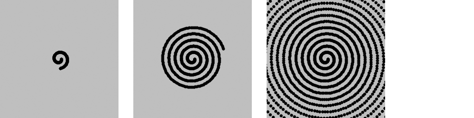
angle=0.0offset=60.0scalar=2.0speed=0.05defsetup():size(120,120)fill(0)defdraw():globalangle,scalarx=offset+cos(angle)*scalar;y=offset+sin(angle)*scalar;ellipse(x,y,2,2)angle+=speedscalar+=speed
Robot 6: Motion

In this example, the techniques for random and circular motion are applied to the robot. The background() was removed to make it easier to see how the robot’s position and body change.
At each frame, a random number between −4 and 4 is added to the x coordinate, and a random number between −1 and 1 is added to the y coordinate. This causes the robot to move more from left to right than top to bottom. Numbers calculated from the sin() function change the height of the neck so it oscillates between 50 and 110 pixels high:
x=180.0# x coordinatey=400.0# y coordinatebodyHeight=153.0# Body heightneckHeight=56.0# Neck heightradius=45.0# Head radiusangle=0.0# Angle for motiondefsetup():size(360,480)ellipseMode(RADIUS)background(0,153,204)defdraw():globalx,y,angle# Change position by a small random amountx+=random(-4,4)y+=random(-1,1)# Change height of neckneckHeight=80+sin(angle)*30angle+=0.05# Adjust the height of the headny=y-bodyHeight-neckHeight-radius# Neckstroke(102)line(x+2,y-bodyHeight,x+2,ny)line(x+12,y-bodyHeight,x+12,ny)line(x+22,y-bodyHeight,x+22,ny)# Antennaeline(x+12,ny,x-18,ny-43)line(x+12,ny,x+42,ny-99)line(x+12,ny,x+78,ny+15)# BodynoStroke()fill(255,204,0)ellipse(x,y-33,33,33)fill(0)rect(x-45,y-bodyHeight,90,bodyHeight-33)fill(102)rect(x-45,y-bodyHeight+17,90,6)# Headfill(0)ellipse(x+12,ny,radius,radius)fill(255)ellipse(x+24,ny-6,14,14)fill(0)ellipse(x+24,ny-6,3,3)