Three

Classical Open-population Capture–Recapture Models

KENNETH H. POLLOCK AND RUSSELL ALPIZAR-JARA

3.1 Introduction

In the previous chapter closed capture–recapture models were considered for situations where the population size does not change during the study. When open-population models are used, the processes of birth, death, and migration are allowed, and therefore the population size can change during the study. Studies of open populations often cover extended time periods, and the population changes that occur are of great interest to ecologists and managers. The most popular model of this open model class is the Jolly-Seber (JS) model (Jolly 1965; Seber 1965, 1982; Pollock et al. 1990; Schwarz and Seber 1999), which requires that the number of uniquely marked and unmarked animals be recorded on each trapping occasion. Therefore, a complete capture history of each captured animal is available. The model allows estimation of the parameters pertaining to population sizes, survival rates, recruitment numbers, and capture probabilities. However, it is not possible to separate survival from emigration or recruitment from immigration without additional information.

There were early open-population capture–recapture models of importance when they were developed (e.g., Jackson 1939, 1940, 1944, 1948; Fisher and Ford 1947; Leslie and Chitty 1951; Leslie et al. 1953). Entomological research was the motivation for some early model development. Jackson developed early models to study tsetse fly populations in Africa, and R. A. Fisher developed models to help E. B. Ford study a moth population. These models did not handle variability correctly. They were either deterministic or partially deterministic, and underestimated the variances of estimators (Cormack 1968). These models have been superseded by the stochastic Jolly-Seber model and should no longer be used.

Two papers that appeared before the papers of Jolly (1965) and Seber (1965) stand out as crucial to the development of the JS model. In the first, Darroch (1959) presented maximum likelihood estimators for two special cases of the open-population model. These were the additions-only model (only births and immigration allowed) and the deletions-only model (only deaths and emigration allowed). Pollock (2001) in a paper discussing Seber’s contributions to the field notes that it was actually Darroch who introduced Seber to capture–recapture models. That turned out to be a very fortunate personal connection for the development of the field!

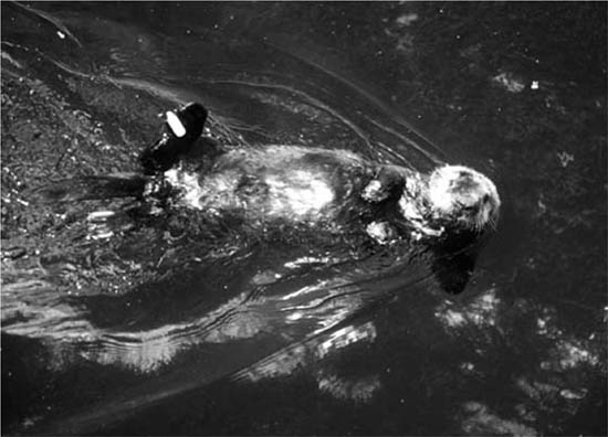
Figure 3.1. Flipper-tagged sea otter (Enhydra lutris), Monterey Bay, California, 1995. (Photo by Steven C. Amstrup)

The second crucial paper was by Cormack (1964). He considered survival and capture probability estimation for marked birds and derived one component of the likelihood used by Jolly and Seber in their more general model. To recognize Cormack’s contribution to development of these models, most scientists now use the term Cormack-Jolly-Seber (CJS) model when referring to the marked animal component of the likelihood function (e.g., Lebreton et al. 1992).

The work of Jolly and Seber has had a tremendous impact in the development of open capture–recapture models. See Seber (1982, p. 196) for an excellent detailed description of the Jolly-Seber model and Pollock et al. (1990) for a comprehensive exposition with several illustrative examples and some model restrictions and extensions. Many new models have followed from this seminal work and these will be presented in later chapters of this book.

In this chapter we discuss the original JS model, its relationship to the CJS model, and some restricted and more generalized versions of the JS model. This is followed by a discussion of age-dependent models, including one proposed by Manly and Parr (1968). General issues of model selection and goodness of fit are considered next, followed by the illustration of the methodology with a comprehensive example.

3.2 The Original Jolly-Seber Model

The following notation consistent with standard usage and table 1.1 of chapter 1 is used in this chapter. Parameters are

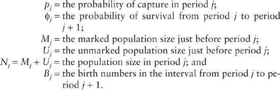
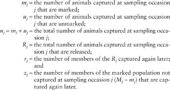
Statistics are

Parameter Estimation

We now present an intuitive derivation of parameter estimates for the standard Jolly-Seber model where capture and survival parameters are allowed to vary in each period. These estimates are based on a maximum likelihood (ML) approach (Seber 1982, p. 198; chapter 1 this volume). While in practice one would obtain the ML estimates using a computer program like JOLLY (Pollock et al. 1990), POPAN (Arnason and Schwarz 1999), or MARK (White and Burnham 1999), we believe these intuitive estimates can help biologists to understand the structure of the (JS) model and also see more clearly why the various assumptions made are so crucial.

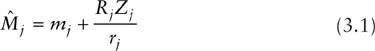
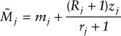
All of the necessary estimators rely on the estimation of the marked population size, M_j. Because deletions (deaths and emigration) are possible under open models, M_j must be estimated. This is done by equating the future recapture rates of two distinct groups of animals in the population at time j: (1) those that are already marked but not seen at time j(M_j − m_j), and (2) those that are seen and released at time j (R_j). Under the assumption of equal catchability of individuals, the future recapture rates of these two groups should be equivalent. Thus, if z_j and r_j are the members of the M_j − m_j and R_j that are captured again later (at least once), then

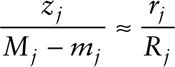
and

for j = 2, …, k − 1.

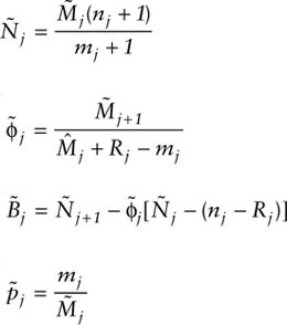
The “survival” rate estimator is obtained from the ratio of marked animals present at time j + 1 to those present at time j,

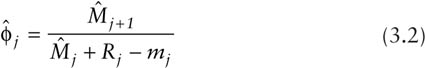
for j = 1, … , k − 2, where the term, R_j − m_j, represents the number of newly marked animals released at time j. The survival estimator does not distinguish between losses due to death and permanent emigration without more information. Therefore, this quantity is often called “apparent survival” in the literature.

The capture probability, p_j is estimated as the ratio of marked animals caught at time j to the number present in the population at time j:

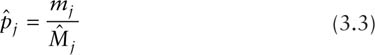
for j = 2, 3, … , k − 1.

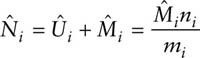
The population size for period j can be determined by equating the sample and population ratios of marked to total animals,

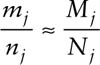
and then, just as with the Petersen-Lincoln estimator,

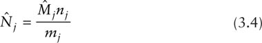
or

Here, n_j represents the number of animals captured at each sampling occasion, m_j of which are marked.

To estimate birth numbers, the difference in population size at time j + 1 and time j is determined, accounting for deaths due to natural mortality (1 − ϕ_j) and capture mortality (n_j − R_j):

for j = 2, … , k − 2. The “birth” number estimator cannot distinguish between individuals entering the population due to recruitment and immigration. This reflects the fact that this estimator for birth is derived purely by subtraction and has nothing to do with the actual processes surrounding birth. Although it has to be considered a poor estimator for recruitment, as opposed to other processes that can bring new animals into a population; it may be possible to separate individuals entering a sample on the basis of their size, sexual maturity, etc. and thereby informally test whether it is indicative of actual births. Negative estimates for this quantity are possible in practice, especially if population sizes and capture probabilities are low (see table 3.3 in the Example in section 3.7 below). Such estimates should be set at zero because there cannot be “negative” births.

The Jolly-Seber model also allows estimation of the probability of an animal being returned to the population in sampling occasion j by R_j/n_j. Its complement estimates the proportion of animals lost on capture.

All of the above estimators are subject to small sample bias, but Seber (1982, p. 204) gives approximately unbiased versions that are as follows:

and

The estimated variances and covariances of all these estimators, based on asymptotic theory, are presented by Seber (1982, p. 202) and Pollock et al. (1990). Here we present only the estimated variance for the population size estimate, which is

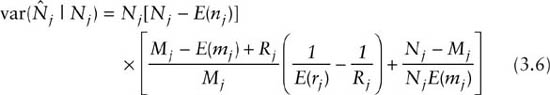
and the total variance for the survival estimate

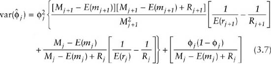
Because estimates of birth are linked to estimates of survival by simple subtraction (equation 3.5), estimates of survival rates and recruitment numbers can be negatively correlated. Estimates of these parameters should be interpreted with this in mind. Generally, for small samples, estimated variances tend to be smaller than the true variances.

Assumptions

Many assumptions need to be made for the Jolly-Seber model to be valid and for the estimators to be approximately unbiased:

1. every animal alive in the population at a given sample time j has an equal chance (p_j) of being captured in that sample (equal catchability);

2. every marked animal alive in the population at a given sample time j has an equal chance of survival (ϕ_j) until the next sampling occasion (implicitly, this assumption applies to all animals, marked and unmarked, in order to estimate the survival of all animals in the population);

3. marked animals do not lose their marks and marks are not overlooked;

4. sampling periods are short (i.e., effectively instantaneous); and

5. all emigration from the population is permanent.

Properties of Estimators

Pollock et al. (1990) stated that population size estimates are negatively biased (i.e., tend to be too small) by heterogeneity of capture probabilities. This is similar to the situation with closed models that make this assumption (chapter 2 of this volume). Population size may be positively or negatively biased by permanent trap response (chapter 2 of this volume). If animals are trap happy then there is a negative bias, whereas if animals are trap shy then there is a positive bias. Temporary changes in capture rate after marking (i.e., temporary trap response) can be detected and then estimated using the models of Robson (1969), Pollock (1975), and Brownie and Robson (1983).

Survival estimates are relatively robust to heterogeneity of capture probabilities. They also are not affected by trap responses, although measures of precision are affected, depending on the type and magnitude of the violation. With trap-happy animals precision is improved, while for trap-shy animals precision is lessened (Pollock et al. 1990).

Survival probabilities may also be heterogeneous in the population. Pollock et al. (1990) discuss this in some detail. If the same animals tend to have higher or lower survival probabilities consistently from year to year then both survival-rate estimates and population size estimates are positively biased. The situation is still more complex if survival and capture probabilities are both heterogeneous at the same time, a situation that still requires more research. See Pollock and Raveling (1982) and Nichols et al. (1982b) for details in the related setting for band-recovery models.

If marking influences survival, which unfortunately sometimes occurs in practice, then survival rates can be severely underestimated and population sizes will have a positive bias that can also be severe. Some methods of marking fish suffer from this problem (Ricker 1958; Pollock et al. 1990; Hoenig and Pollock, chapter 6 this volume). Temporary reductions in survival rate after marking can be detected and then estimated using the models of Robson (1969), Pollock (1975) and Brownie and Robson (1983).

Any loss or overlooking of tags will result in overestimation of population size in open models, especially if the capture probability is low (McDonald et al. 2003). Survival estimates will be negatively biased by tag loss (Arnason and Mills 1981). Clearly, the choice of tag type (dye, fin clip, ear tag, radio collar, etc.) is important. Double marking schemes can be used to estimate tag loss and adjust for it (Seber 1982, p. 94). Given recent improvements in sighting technology, distinctive natural features of individuals have sometimes been used as natural marks (e.g., see Karanth and Nichols 1998; and Smith et al. 1999).

It is important to emphasize that the positive biases in population sizes, due to tag-loss or tag-induced mortality reported here, are different from the results presented in Pollock et al. (1990, pp. 25–26). They stated that tag loss or tag-induced mortality would not cause a bias in population size estimates. This result was based on large sample arguments, and also assumed that the tag loss rate or tag-induced mortality rate was homogeneous over time. Clearly a realistic model for tag loss would be heterogeneous with some tags lost quickly and some others lost at a slower rate. Under such a model tag loss does cause a serious positive bias unless the capture probability is high as stated previously. A similar argument applies to tag-induced mortality (McDonald et al. 2003).

The assumption of instantaneous sampling periods is important because otherwise animals would have to be assumed to have survived from the midpoint of one sampling interval to the midpoint of the next sampling interval. Animals captured toward the end of the sampling interval would actually have to survive less time to the next sampling interval. This would cause some heterogeneity of survival probabilities but in practice this should not be serious. Sampling periods are never instantaneous, but certainly sampling periods should be kept as short as possible.

Emigration must be permanent for the JS model to be valid. Recall that estimation of the number of marked animals involved using the z_i (animals captured before and after i but not at i), and it is important that these animals be present at time i when they were not captured. Temporary emigration may occur in practice and can be extremely important but this is not discussed until chapter 5.

Pollock et al. (1990, p. 70) present a discussion of precision of the JS estimators. They include some graphs to aid the reader. However, simulation can always be used to study their particular cases in detail. The computer packages MARK and POPAN both include simulation capabilities. Precision is influenced by many factors, such as the number of captured individuals, capture probabilities, and the degree of capture probability heterogeneity. However, in general terms, survival rates and population sizes can be estimated reasonably well, but birth numbers have poor precision unless the capture probabilities are extremely high (Pollock et al. 1990, figure 8.10).

3.3 The Jolly-Seber Likelihood Components

Traditionally the JS model has been based on a maximum likelihood approach to estimation (see chapter 1). Despite the fact that they obtained the same point estimates of the parameters presented earlier, Jolly (1965) and Seber (1965) used different likelihoods. Here the approach of Seber (1982) and Brownie et al. (1986) is used to explain the components of the likelihood. Crosbie and Manly (1985) and Schwarz and Arnason (1996) use a different formulation that handles the birth process in a more elegant manner, as discussed in chapter 5.

The likelihood can be viewed as three conditionally independent components with the overall likelihood the product of these, i.e., L = L₁ · L₂ · L₂. The first component, L₁, is a product binomial likelihood that relates the unmarked population and sample sizes at each time to the capture probabilities. The second component, L₂, will not be discussed further here. The only parameters it contains are the probabilities of being lost on capture. The third component, L₃, is the component that contains all the recapture information conditional on the numbers of marked animals released each time. The only parameters contained in this component are the capture and survival probabilities. This is the CJS likelihood that was originally derived by Cormack (1964).

One way to view estimation in the full JS model is that capture and survival probabilities (and marked population sizes) are estimated from L₃. The nuisance probabilities of losses on capture are estimated from L₂, and the unmarked population sizes estimated from L₁. The estimate of the unmarked population takes the form

The estimate of population sizes then follows and is the same as that derived earlier in equation 3.4, namely

Note that in this formulation the population sizes and birth numbers do not appear in the likelihood directly and are derived parameters.

The Cormack-Jolly-Seber Model

In some cases all components of the likelihood are combined in the general JS model as we just described. However, in other cases the CJS model may be used alone to estimate survival and capture probabilities (Cormack 1964). This CJS model requires information on only the recaptures of the marked animals, and that the marked animals be representative of the population. In some cases the marking process may use a totally different method of capture than the recapture process, as with mark–resight studies. See, for example, Pollock et al. (1990, p. 51) for a description of a mark–resight study on Canada geese. The dependence, in the CJS model, on only recaptures of marked animals means that population size cannot be estimated directly.

The original CJS model was for one group of animals and assumed no age-dependence of survival and capture probabilities. Lebreton et al. (1992) presented a unified approach to extensions of these models that allows modeling of survival and capture (sighting) probabilities as function of time, age, and categorical variables characterizing the individuals. This is discussed in chapter 5.

3.4 Restrictions and Generalizations of the Jolly-Seber Model

Various restricted versions of the general JS model have the substantial advantage of reducing the numbers of parameters to be estimated. The deaths-only model may sometimes be useful if there is no immigration and recruitment is not occurring. Similarly the births-only model may sometimes be useful if there is no mortality or emigration (Darroch 1959). Both restricted versions of the general model are implemented in the computer program JOLLY. Versions of the general model with the restrictions of constant survival and/or capture probabilities were developed by Jolly (1982) and Brownie et al. (1986), and they have also been implemented in JOLLY. They will be illustrated by an example later.

Generalizations of the JS model that allow for temporary effects on survival and capture rates have been considered. Temporary reductions in survival rate after marking and temporary changes in capture probability can be detected and then estimated using the models of Robson (1969), Pollock (1975), and Brownie and Robson (1983). Some of these models have also been implemented in JOLLY and they can easily be implemented in MARK.

3.5 Age-dependent Models

Generalizations of the JS model such as those allowing age dependence are also possible. Early work was by Manly and Parr (1968), whose model also illustrates some features of the JS model. As we discussed earlier, the estimator of population size in the JS model can be written

with the estimator of capture probability given by

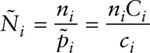
Manly and Parr (1968) realized that one could estimate p_i in a manner that was robust to heterogeneity of survival rates due to age and came up with a different estimator. They defined C_i as the class of marked animals known to be alive at time i because they were captured before and after i, and they defined c_i as the members of that class C_i that are captured at i. Therefore, an estimate of p_i is

and hence

A Chapman modification to reduce bias is then

Also survival rate and birth numbers can be estimated as described in Seber (1982, p. 236). We believe all these estimators will have larger standard errors than the Jolly-Seber estimators because they use a smaller class of marked animals (C_i) as the basis of their estimation rather than the total marked population (M_i). However, this model has not been much studied, and Seber (1982, p. 234) presents only an approximate variance for the population size estimators. In section 3.7 we present a small example and contrast the Manly-Parr estimates with the JS estimates.

There has been much work on age-dependent models. A focus of particular interest has been the situation when more than one identifiable age class is marked (Pollock 1981a; Pollock and Mann 1983; Stokes 1984; Loery et al. 1987; Pollock et al. 1990). This research led to the computer program JOLLYAGE. Recently MARK (White and Burnham 1999) has made many of these analyses very easy to perform, as considered further in chapter 5.

3.6 Goodness-of-Fit and Model Selection Issues

There are two aspects to assessing whether the best model for an open capture–recapture model has been chosen. There is the overall goodness of fit of a model, and the decision about which of a series of related models is the best. Some of this material has been discussed in chapter 1, and only a very brief summary is presented here.

Assumption violations may mean that a model does not fit the capture–recapture data available. Seber (1982, p. 223) suggested the standard chi-squared test based on comparing observed and expected values for assessing the general JS model. Pollock et al. (1985) derived two related tests based on minimal sufficient statistics. Each chi-squared test had two contingency tables based on conditional arguments and sufficient statistics for the general JS model. Brownie et al. (1986) extended these goodness fit tests to the restricted models B (constant survival) and D (constant survival and constant capture). All of these tests are implemented in JOLLY and are used in an example that follows.

Traditionally likelihood ratio-type tests have been used to choose which model to fit from a nested set (chapter 1). Brownie et al. (1986) used a related approach based on conditional sufficient statistics to compare models, and these have been implemented in JOLLY. There is an example in section 3.7. The modern approach to testing between models is to use the AIC procedure described briefly in chapter 1. It allows the comparison of nonnested models, and puts a penalty on fitting a model with too many parameters. The AIC method is used with the CJS example using MARK presented below.

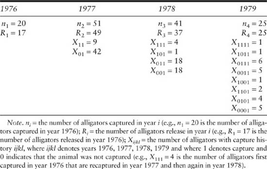
TABLE 3.1
Alligator between-year capture-history data collected by Fuller (1981) for a population at Lake Ellis Simon, North Carolina, from 1976 to 1979

3.7 Examples

A Jolly-Seber Example

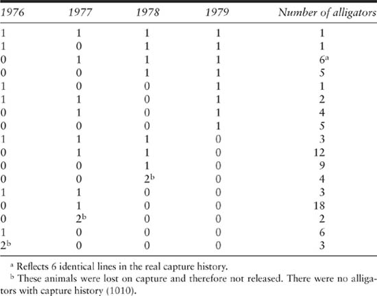
To illustrate the calculation of statistics and parameter estimation we use data from a capture–recapture study on a population of the American alligator (Alligator mississippiensis) at Lake Ellis Simon, North Carolina, between 1976 and 1979 (Fuller 1981). This data set has been previously analyzed to illustrate the advantages of Pollock’s robust design in capture–recapture experiments, and is directly taken from Pollock (1982, p. 756) and Pollock et al. (1990, p. 60). This data set is small enough so that it is easy to handle the computations with a calculator. The estimation of parameters with larger data sets is practical only with the use of computer programs that are readily available, such as JOLLY, POPAN, or MARK. The capture-history data are presented in table 3.1 and the capture-history matrix in table 3.2. The data are analyzed first by doing the direct calculations for the full model, and then with the program JOLLY using the data as presented in table 3.2. There was an error in the data as originally published, and X₁₀₀₁ = 1 and not 0.

TABLE 3.2
Capture-history matrix for the Jolly-Seber model (JOLLY) and the Cormack-Jolly-Seber model (MARK)

By definition m_i = the number of marked animals captured in the ith sample (i = 2, … , k). Also, from table 3.1,

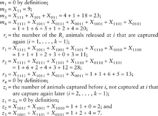
Based on these summary statistics the bias adjusted parameter estimates can be obtained. Bias-adjusted estimates can also be computed using program JOLLY with model A, and the standard errors reported here are from the output from this program.

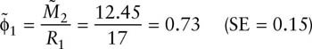
First note that we can estimate the marked population sizes for years 2 and 3, so that

and

Also, survival rates for year 1–2 and year 2–3 are

and

Notice that the estimates of survival are quite similar. The relative precision of an estimate (the coefficient of variation, CV) is the standard error divided by the estimate itself. The CVs in the present case 0.15/0.73 and 0.15/0.80, respectively, or 20.5 and 18.7%, respectively. This level of precision is quite reasonable in wildlife science.

It is possible to estimate the population sizes in years 2 and 3, so that

and

The relative precisions for the population size estimates are similar to those for the survival estimates, at approximately 20%.

The capture probabilities for years 2 and 3 are

and

For this small example with four sampling periods it is possible to estimate only one set of birth numbers, for the period between years 2 and 3:

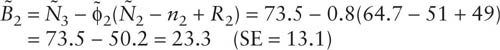
This estimate has poor relative precision (13.1/23.3, or 56.2%). Poor precision for estimates of birth numbers is common in practice (Pollock et al. 1990, p. 71).

Restricted Parameter Model Output from Program JOLLY

Jolly (1982) showed that when restricted models (with the assumptions of constant survival and/or capture probabilty over time) are reasonable, then there can be a large gain in the precision of estimators compared to the standard JS estimators because these parsimonious models have many fewer parameters. Of course, if the assumptions of constancy of survival or capture probability are not valid then bias will be introduced. Program JOLLY offers features such as maximum likelihood parameter estimates, goodness-of-fit tests, and methods to aid in model choice based on likelihood ratio-type tests, but the newer AIC method of model choice is not available. The calculations above suggest that the survival rates for year 1–2 and year 2–3 are very similar. Hence, it may be useful to test the assumption of equal survival rates to reduce the number of model parameters and gain some precision in the estimates. Consider two restricted versions of the original JS model that are implemented in the program JOLLY. These are model B, which assumes that survival probabilities are constant over the whole experiment (i.e., ϕ₁ = ϕ₂ = ϕ₃), but capture probabilities may vary from year to year, and model D, which assumes that both the survival and capture probabilities are constant over the whole experiment (i.e., ϕ₁ = ϕ₂ = ϕ₃ and p₂ = p₃ = p₄). Table 3.3 shows the parameter estimates for the three models A, B, and D.

TABLE 3.3
Estimates and approximate standard errors (in parentheses) under the Jolly-Seber model (A), the constant survival model (B), and the constant survival and capture model (D) for an alligator population at Lake Ellis Simon, North Carolina, from 1976 to 1979

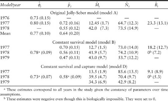
Table 3.4 presents a summary of omnibus goodness-of-fit tests and tests comparing models. This can be used to aid in model selection. Small significant p values indicate a lack of fit, so that the three models all fit the data reasonably well. However, a nonsignificant goodness-of-fit test does not necessarily guarantee that all the model assumptions are met, because these tests may have low power. The other likelihood ratio-type tests are used for comparing two models, with the simpler model being the null and the more complex model the alternative. Small p values suggest that the null model should be rejected. Here none of the likelihood ratio-type tests are significant at any reasonable level. This suggests, following the principle of parsimony (choose an acceptable model with the smallest number of parameters), that the model D estimates are the best as a summary of the population.

Model D seems rather restrictive biologically and the time-dependent estimates of capture in model A do appear to vary quite a lot. This is a small example and another more complex model may have been chosen if there had been more animals marked and recaptured. Note that model B and model D allow the estimation of additional parameters when compared to the full JS model. Negative birth numbers estimates are possible in these models and they occur for both model B and model D. These have been set to zero, as clearly such estimates are biologically impossible.

TABLE 3.4
Tests for the Jolly-Seber model (A), the constant survival model (B), and the constant survival and capture model (D) for an alligator population at Lake Ellis Simon, North Carolina, from 1976 to 1979

In 1978 it is estimated that there were about 70 animals (SE = 9.7) from model D. In that year it was possible to carry out a closed-population analysis and it was estimated that there were about 140 animals (SE = 28.5) using model M_h, the heterogeneity model (Pollock 1982). There is a large discrepancy in the estimates; and even though the standard errors are large there appears to be something else important going on. It is suspected that there was substantial heterogenity of capture probablities due to the large size range of the alligators considered, and that this caused a negative bias in the population size estimates. The so-called robust design allows for this problem and will be discussed in chapter 5. Notice that the goodness-of-fit tests did not pick up this important problem, probably because this is a small population with only four years of data, and therefore the tests have low power (Pollock et al. 1990).

Cormack-Jolly-Seber Component Example in MARK

The CJS model allows the estimation of capture and survival rate estimates, based on the recapture component of the likelihood, using the capture history data in table 3.2 and the recaptures-only option in MARK. The data format had to be modified slightly from that used for JOLLY, but the data were the same. The first step was to use the model-selection procedure to decide on a parsimonious model using the AIC criteria, as discussed in chapter 1. Four models were considered, where survival was either varying over time (ϕ(t)) or constant over time (ϕ(·)) and capture probability was also either varying over time (p(t)) or constant over time (p(·)). The simplest model has two parameters (ϕ, p) and the full model has five parameters (ϕ₁, ϕ₂, p₂, p₃, ϕ₃p₄). It is not possible to separately estimate the last survival and capture probability parameters. The other two models have 4 parameters (3 capture probabilities and 1 survival probability, or 3 survival probabilities and 1 capture probability). In this case the winner in terms of minimum AIC is the simplest model with both capture and survival constant over time (table 3.5). This is the same result as was obtained with the program JOLLY but that older program does not use the AIC criteria.

TABLE 3.5
Program MARK AIC model comparisons for an alligator population at Lake Ellis Simon, North Carolina, from 1976 to 1979

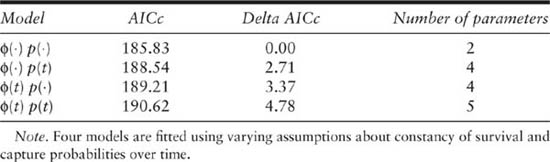
The estimates of constant survival and capture probabilty were = 0.73 (SE = 0.08), and = 0.58 (SE= 0.10), respectively. These estimates are the same as those reported in table 3.3 for model D using program JOLLY, but there are small differences in the standard error estimates due to the different algorithms used for the calculations.

Manly-Parr Example

Table 3.6 shows Manly-Parr estimates for the alligator data, based on the equations in section 3.5. The calculations at the base of the Manly-Parr method for time 2 are the total number of marked animals known to be alive at time 2 (C₂), and the number of those captured (c₂). These are

and

Similar calculations for time 3 give C₃ = 15 and c₃ = 8.

TABLE 3.6
Comparison of Manly-Parr and Jolly-Seber parameter estimates for the alligator data at Lake Ellis Simon, North Carolina, from 1976 to 1979

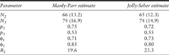
The estimates of the Manly-Parr method for population size, capture probability, survival rate, and birth number can be obtained using the equations given in the previous section. These estimates allow for age-dependent survival rates. Table 3.6 also compares these Manly-Parr estimates to the JS estimates calculated previously, and in this case all of the estimates are very similar. The standard errors for the population size estimates are slightly larger for the Manly-Parr method, as expected because it uses the data in a less efficient way.

3.8 Conclusions

The Jolly-Seber capture–recapture model is important because the estimation of survival, birth numbers, and population sizes is done in one analysis, based on a well-defined stochastic model. However, one major problem with these models is that unlike the closed capture–recapture models they do not allow for unequal catchability of individual animals due to heterogeneity or trap response. In chapter 5, a solution to this problem is given, together with the development of many other new methods based on the original JS model.

3.9 Chapter Summary

• The early history of models for open-population capture–recapture data is reviewed, leading up to the stochastic models of Darroch, Cormack, Jolly, and Seber.

• The Jolly-Seber model is described, with intuitive explanations for the estimators of survival probabilities, capture probabilities, population sizes, and birth numbers. Equations for the variances of the estimators of population size and survival probabilities are provided. The assumptions needed for the use of the model are discussed, together with the general properties of the estimators.

Figure 3.2. Jerry Hupp prepares to release a Canada goose (Branta canadensis) after surgical implantation of a VHF radio-transmitter, Anchorage, Alaska, 1999. Also note the double leg bands. (Photo by John Pearce)

• The components of the likelihood function for the Jolly-Seber model are defined. Components of the Cormack-Jolly-Seber model, which is conditional on the first releases of marked animals, are also defined.

• Restrictions and generalizations of the Jolly-Seber model are discussed.

• The models of Manly and Parr and others allowing for parameters to vary with the age of animals are discussed.

• Tests for goodness of fit and model selection are briefly reviewed.

• The Jolly-Seber method is illustrated using data from a study of the American alligator. The same data are then analyzed using models that assume that the probabilities of capture and/or the probabilities of survival are constant.

• The use of the Cormack-Jolly-Seber model for the same data is illustrated using the program MARK. The Manly and Parr estimates are also shown.