
Chapter 7. Machine Learning and Differential Privacy
Machine learning is a term that describes a variety of tools to find patterns in data. In this chapter, you will learn the basics of machine learning, using linear regression as an entry point. Building upon this knowledge, you will learn about the relationship between the training process, model parameters, and potential privacy violations. To defend against different attack scenarios you will learn about different ways to privatize machine learning models during the training process.
Broadly speaking, machine learning is the process of a computer receiving a data set and learning relationships and patterns in it. The process of learning these patterns is called training. Given a function with some unknown parameters, the training process tries different parameter values until it finds the values that allow it to most closely match the data. In order to understand how accurate the model is, you perform testing - this is the part of the process where you use your parameters to make predictions based on the input data, and compare the predictions to the true values. If the tests show that your model is accurate, then congratulations, you’ve trained the computer to learn a model about the data. If not, it is back to the drawing board, but there are always other model types and training processes to try.
For example, simple linear regression is a process that estimates the slope and intercept between two columns in a dataset. These two parameters uniquely determine a line in the plane that estimates a linear relationship in your data set. This seems innocuous enough, however, there are situations in which you will need to privatize this model in order to protect the privacy of individuals in the training data.
Why would you need to do this? Consider a membership attack 1 where a malicious actor observes that a model is more confident about its prediction on certain data points. The actor can then conclude that these points are similar to the points that the model was trained on. By repeatedly tuning these data points to maximize the model’s confidence, the actor can converge on points that are very close (or identical) to real data points from the training set. In cases where a model was trained on sensitive data, this constitutes a privacy violation. 2.
Supervised vs. Unsupervised Learning
Machine learning is often broken into two broad categories: supervised, and unsupervised. Supervised learning describes a scenario where the data comes with labels to learn from. These labels aid the model in learning patterns between the different categories. For example, the following table shows a data set of fruit measurements.
Height (cm) | Diameter (cm) | Type |
6.2 | 6.7 | Apple |
7.0 | 6.9 | Orange |
9.0 | 6.2 | Pear |
6.3 | 6.5 | Apple |
7.1 | 6.8 | Orange |
6.4 | 6.8 | Apple |
9.1 | 6.1 | Pear |
9.2 | 6.2 | Pear |
7.2 | 7.4 | Orange |
Now imagine you are given a task - you know the height and circumference of a fruit, and want to predict its type. In this case, the column Type is the label of the data set - it is what your model wants to predict. This is an example of supervised learning - the word supervised is used here because you are “supervising” the model’s learning process by giving it labels to learn from. Supervised learning is common in scenarios where you have large amounts of pre-existing data that was labelled by humans.
If, on the other hand, you are given the dataset without this column, then your learning objective is different.
Height (cm) | Diameter (cm) |
6.2 | 6.7 |
7.0 | 6.9 |
9.0 | 6.2 |
6.3 | 6.5 |
7.1 | 6.8 |
6.4 | 6.8 |
9.1 | 6.1 |
9.2 | 6.2 |
7.2 | 7.4 |
You know that each row represents a fruit, but do not know which type it is. In fact, this data doesn’t even tell you how many types of fruit there are in the data set. With a data set like this, you can perform an unsupervised learning process, which will try to infer how many categories there are in the data, and which category each member belongs to. Thus, it may notice that there are three fruits in the data set where the ratio of height to diameter is large - the fruit is taller than it is wide. These rows will be clustered together and the model will tell you “these objects seem similar.” The model can therefore identify pears based on height and diameter without even knowing what a pear is, it simply looks at patterns in the data and makes its best estimate.
Unsupervised learning is more common in cases where you have data that hasn’t been human reviewed. Sometimes, you will want to understand the global structure of the data as a first pass before doing further analysis on it. In a case like this, unsupervised learning can be a helpful first step to estimate how many clusters exist in the data. In other cases, the unsupervised learning is the main event - a classic example being handwritten digit detection that clusters images of digits into like categories, without any pre-existing labels or human guidance.
Simple Linear Regression
If training a model is the process of making it represent the data as accurately as possible, then how do you measure the correctness of its estimate? You need a mathematical formulation of correctness for the model to compare itself against. Such a formulation is often called an objective function - a function that takes a data point as input, and returns how close the model’s prediction is to the true value.
A simple linear regression model transforms a single argument
Given a set of points
Unfortunately, like any other statistic, regression parameters contain private information about the underlying dataset.
DP Approach 1: Sufficient Statistics
When the data is centered around zero, the regression parameters become relatively simple:
The naive approach is to try to add noise directly to
If all
A common approach to avoid the issue of undefined sensitivity is to replace individual point estimates in the formula, and then postprocess to get an estimate of the final statistic.
Denote the DP estimate for
The sensitivity of
We first consider the case where one record is added:
This derivation makes use of an assumption that all
Now that you have the sensitivities of each of your point estimates
importnumpyasnpfromopendp.measurementsimportmake_base_laplacefromopendp.modimportenable_featuresenable_features("contrib")defdp_beta1_via_plugin(x,y,b,epsilon):x,y=np.clip(x,-b,b),np.clip(y,-b,b)# noise scale is multiplied by 2 to account for the composition# both dp estimators happen to share the same noise distributionlaplace_mech=make_base_laplace(scale=2.0*b**2/epsilon)# make the point releasesdp_Sxy=laplace_mech(sum(x_i*y_iforx_i,y_iinzip(x,y)))dp_Sxx=laplace_mech(sum(x_i**2forx_iinx))# post-processreturndp_Sxy/dp_Sxx
The total privacy expenditure is the basic composition of the privacy expenditure for releasing
Multivariate Regression
The concepts behind simple linear regression can be extended for when you have multiple predictors,
letting
This time, consider a private dataset consisting of m predictors for y.
You would like to solve for
The ordinary least squares solution for estimating a linear regression model is
This formula is a generalization of the univariate case above, where X is the design matrix, with two columns:
-
a column of ones to estimate the bias term
-
the input vector x
Then the quantity
This statement simplifies, since each value in the resulting matrix can be expressed as a sum:
Recall that the inverse of a 2x2 matrix
and we can use this statement to calculate the inverse of
To complete the estimator, we need to calculate
Using the previous definitions of
This simplifies to:
DP Approach 2: Theil-Sen Estimator
Another approach for estimating DP regression coefficients is via a privatized version of the Theil-Sen estimator. The Theil-Sen estimator first makes a random pairing of each point with another point in the dataset. A slope is computed for each pairing, and the median of this set of slopes is used as the final estimate of the slope.
This algorithm is amenable to differentially private techniques, by breaking it into three pieces
-
a transformation from your dataset to a dataset of pairs
-
a transformation from a dataset of pairs to a vector of slopes
-
a DP median mechanism on the vector of slopes
If you plot the dataset of pairs, it looks like this:
importmatplotlib.pyplotaspltimportnumpyasnpdataset_size=20x=np.random.normal(size=dataset_size)y=x*np.random.normal(loc=1.,scale=0.4,size=dataset_size)+3dataset=np.stack([x,y]).T# Randomly construct pairingsnp.random.shuffle(dataset)# This assumes that dataset size is even:dataset_of_pairs=np.array(np.array_split(dataset,2))forp1,p2inzip(*dataset_of_pairs):slope=(p1[1]-p2[1])/(p1[0]-p2[0])plt.plot([p1[0],p2[0]],[p1[1],p2[1]],label=f"{slope:.2f}")plt.legend()plt.show()
The legend shows the corresponding dataset of slopes.
First, consider the stability of a dataset transformation to a dataset of pairs. If an individual may influence at most k records in the input dataset, then in the worst case, the individual may influence up to k pairs.
The transformation from a dataset of pairs to a dataset of slopes is a stable row-by-row transformation. Therefore, it can be argued formally that if an individual can influence at most k records in the input dataset, then the individual can influence at most k slopes.
The final step to estimate
Gradient Descent
Training a machine learning model is fundamentally about minimization. At each step of the training process, the model tries a set of predictions, and calculates error from the true values. It then modifies its parameters and tries again. How does it modify the parameters? By taking a step in the direction of fastest change.
Think of yourself at the top of a mountain. If you want to get to the bottom as quickly as possible, do you zigzag left and right as you do, or do you follow the pull of gravity and walk straight down? Conversely, if you are at the edge of a canyon and want to find the lowest point, you will also walk straight down the side of the canyon, rather than running laps around its edge as you descend.
What is the connection between canyons and machine learning? In this case, if you construct an error function that gives you the difference between your model output and true values, you want to find the parameters that minimize the error. This is a crucial concept moving forward - machine learning is about optimizing parameters that minimize the error between the model prediction and the true values in the data. Ideally, this function should be convex, that is, have only one minimum value. In practice, this isn’t always the case, and there may be multiple local minima in the error function.
For example, consider the function
An implementation of this algorithm is included below.
In this case, the code will only stop iterating once the difference in f changes by an amount specified by the variable
tol.
In other cases, you may want to set a fixed number of iterations in a for loop.
importnumpyasnpdeff(x,y):return(x-2)**4+(y+3)**2defgradient(x,y):returnnp.array([4*(x-2)**3,2*(y+3)])if__name__=='__main__':x_old=10y_old=10gamma=0.01tol=1e-16x_new,y_new=np.array([x_old,y_old])-gamma*gradient(x_old,y_old)whilenp.abs(f(x_new,y_new)-f(x_old,y_old))>tol:x_new,y_new=x_old,y_oldx_old,y_old=np.array([x_old,y_old])-gamma*gradient(x_old,y_old)(x_new,y_new,f(x_new,y_new))
If you run this code, you will see the x and y values descend from 10 down to values increasingly close to 0. Change the gamma value - what do you see?
The following table demonstrates gradient descent for the function, as it searches from the point (1,1) to approximate the minimum at (1.806, -2.994).
| header | x | y | f(x,y) |
|---|---|---|---|
0 | 1 | 1 | 17 |
1 | 1.4 | 0.19999999999999996 | 10.369600000000002 |
2 | 1.4864 | -0.44000000000000017 | 6.623182505122199 |
3 | 1.5405919821824 | -0.9520000000000001 | 4.23884851982989 |
4 | 1.5793762594281457 | -1.3616000000000001 | 2.7156567789467383 |
5 | 1.6091436890118227 | -1.6892800000000001 | 1.741325180606942 |
6 | 1.6330279263142091 | -1.951424 | 1.1176472334399676 |
7 | 1.6527957582168578 | -2.1611392 | 0.71821993366425 |
8 | 1.669538055848909 | -2.32891136 | 0.4622857158456387 |
9 | 1.6839733072533936 | -2.463129088 | 0.2982049664192858 |
10 | 1.6965983044406683 | -2.5705032704 | 0.1929411198544475 |
11 | 1.7077698690579728 | -2.6564026163200003 | 0.12535205723685655 |
12 | 1.7177522690816889 | -2.725122093056 | 0.0819041818260867 |
13 | 1.7267462377198413 | -2.7800976744448 | 0.05393228605201927 |
14 | 1.7349075208010498 | -2.82407813955584 | 0.03588693922437874 |
15 | 1.7423591667431255 | -2.8592625116446717 | 0.024213185580110395 |
16 | 1.7491999223731172 | -2.8874100093157375 | 0.016633001413099688 |
17 | 1.7555101204372556 | -2.90992800745259 | 0.011686050476040176 |
18 | 1.761355902914583 | -2.927942405962072 | 0.008435713837441053 |
19 | 1.7667923113881525 | -2.9423539247696575 | 0.006280888062175426 |
20 | 1.7718655885006172 | -2.953883139815726 | 0.0048354790560833725 |
21 | 1.7766149189414302 | -2.9631065118525806 | 0.0038512287335502717 |
22 | 1.7810737650811392 | -2.9704852094820646 | 0.0031682827917619717 |
23 | 1.7852709046944812 | -2.9763881675856516 | 0.0026835201826356826 |
24 | 1.789231246537579 | -2.981110534068521 | 0.0023302563822229865 |
25 | 1.7929764780799733 | -2.984888427254817 | 0.0020652311076308997 |
26 | 1.7965255848863149 | -2.9879107418038537 | 0.0018602623208747828 |
27 | 1.7998952707629081 | -2.990328593443083 | 0.0016968900736663364 |
28 | 1.803100300399119 | -2.9922628747544664 | 0.0015629365939676355 |
29 | 1.8061537809071124 | -2.993810299803573 | 0.0014502949681062403 |
These numbers are in close agreement with our expectation!
Since the function is differentiable, we can know that
Using Gradient Descent to Learn Parameters
In the previous example, you found the point (x, y) that minimized a function f.
In this case, the data points (x, y) were your data - the inputs to your function.
A more useful scenario is finding parameters for a function that minimize error relative to a data set.
This means that instead of finding a point (x, y) that minimizes a function, you will find the parameters
Consider simple linear regression, where you want to learn the best parameters for
where
Since you want to find the best parameters to match the data, you will take the gradient relative to the parameters themselves:
Then at each step, you update the parameters
importnumpyasnp# Prepare a datasetideal_params=[4.,2.,-3.]dataset_size=100# assuming known dataset sizedata_x=np.random.normal(size=[dataset_size,2])data_y=np.hstack([np.ones(dataset_size),data_x])@ideal_params# Discover params via gradient descentnum_steps=10params=np.zeros(3)for_inrange(num_steps):instance_level_grads=gradient(data_x,data_y)# n x 2 arraydf_dx=dp_mean(instance_level_grads[:,0])df_dy=dp_mean(instance_level_grads[:,1])params-=gamma*np.array([df_dx,df_dy])
Stochastic Gradient Descent
While gradient descent is a powerful tool for finding the minimum of a function, it has its limitations. Look back to the gradient calculation step in the previous chapter, and note that it requires iterating over the entire data set for each of the parameters. This is only practical for small data sets over a low number of dimensions. Otherwise, the process can become computationally burdensome.
Imagine you are trying to minimize the error over hundreds of parameters and a data set with millions of entries - this would quickly become untenable. For example, a problem with 100 parameters and a data set of 100,000 rows would mean 100 * 100,000 = 10,000,000 calculations to compute the gradient. Further, this step will often be carried out hundreds or thousands of times in order to converge to an approximation of the minimum. Even 100 steps would mean doing 100 * 10,000,000 = 1 billion calculations! We clearly need something more efficient.
Thankfully, there is a technique called stochastic gradient descent, where the gradient is approximated via a random shuffling of the data. Rather than iterate over the entire data set, this algorithm first randomly permutes the data set, then takes a random sampling of the permuted data. Gradient descent is then performed on this random sample, leading to an approximation of the true gradient. Consider the efficiency challenge mentioned in the previous paragraph - if you have a problem with 100 parameters and 100,000 data points, the total number of calculations needed becomes unreasonable. However, if you take a random sample of 1000 data points and approximate the gradient, your total number of calculations drops from 1 billion to (100 parameters) * 1000 (data points) * 100 (iterations) = 10 million, a substantial improvement in speed over regular gradient descent.
When using multiple small subsets of the data (often called batches), the process is called mini batch gradient descent. In mini batch gradient descent, each iteration involves splitting the data set into multiple small subsets and calculating the gradient for each batch. This technique lends itself easily to parallelization - imagine you have 10 minibatches to calculate gradients over. You can have each calculate in parallel, and then average the results together.
Privatizing the Gradient Descent Process
You are already familiar with the DP concepts necessary to privatize the gradient descent algorithm. In this case, you will just be using the DP mean on each component of the gradient to privatize the training process.
The following code snippet does exactly this - for each iteration of gradient descent, it takes the DP mean of the x component and the DP mean of the y component of the gradient. Then, instead of taking a step in the direction of the gradient, it takes a step in the direction of a vector of these DP means. Think of this like taking little random steps to the left and right as you walk down a hill - it will no longer be the fastest route from top to bottom, but predicting your path will be harder for someone trying to follow behind you.
Minimum Viable DP Gradient Descent
This section demonstrates a rudimentary DP gradient descent algorithm. The presentation here focuses on simplicity at the expense of utility. The next chapter will make adjustments to the algorithm that make it practically useful, by increasing the complexity.
Gradient descent iteratively updates each weight (parameter) in the network:
Where
Based on this formula, each of the parameters in models trained with gradient descent can be decomposed into the sum of some initial random value
Now take a closer look at how to compute a single DP gradient.
In each training step, the gradient is a dataset transformation from a batch of
importopendp.preludeasdpimportnumpyasnpdp.enable_features("contrib")data_size=1_000x=np.random.normal(loc=0,scale=2,size=data_size)y=x*2+3w_slope,w_scale=0.0,0.0learning_rate=0.01num_steps=500input_space=(dp.vector_domain(dp.atom_domain(T=float),size=data_size),dp.symmetric_distance(),)dp_mean=(input_space>>dp.t.then_clamp((-1.0,1.0))>>dp.t.then_mean()>>dp.m.then_laplace(scale=0.5))per_query_epsilon=dp_mean.map(2)foriinrange(num_steps):y_pred=w_slope*x+w_scaleerror=y_pred-yw_slope-=learning_rate*dp_mean(2*x*error)w_scale-=learning_rate*dp_mean(2*error)("params:",w_slope,w_scale)("total epsilon:",per_query_epsilon*2*num_steps)
Unfortunately, implementing this in practice with modern deep learning frameworks is more difficult because they typically do not provide a way to access the gradients corresponding to each individual input (before aggregation). Access to this more granular gradient is necessary for the DP mean because the DP mean needs to clip the gradient before aggregating in order to keep the sensitivity finite. This is one of the motivations for bespoke libraries for differentially private training, like Tensorflow-Privacy and Opacus.
Private Aggregations of Teacher Ensembles
Private aggregations of teacher ensembles (PATE) is a framework to transform any supervised machine learning classification model into a differentially private classification. The PATE framework trains a model on sensitive data without revealing the data itself. There are three main components to PATE:
-
an ensemble of multiple teacher models
-
an aggregation method
-
a student model
PATE involves training multiple models (called teachers) on the same task, and then combining their predictions such that the prediction output is differentially private. The PATE framework starts by dividing the dataset that is available for model training into several data partitions. Each individual data partition is used as a training dataset in a supervised machine learning task. These trained models are called teacher models. When making prediction about an instance x, PATE does the following:
-
For each trained model, get the predictions for the instance x.
-
Count the number of teacher models that voted for each class, creating a histogram of votes for each class.
-
Apply the Laplace or Gaussian Mechanism to the histogram created in the previous step.
-
The output is selected by choosing the class with the highest number of votes from the DP-histogram generated in the previous step.
The following diagram illustrates these steps: the data is partitioned into disjoint subsets, and each is sent to train a different teacher model.

Figure 7-1. Differentially private classification with PATE framework.
First, multiple models are trained on different disjoint subsets of the data - these are called teacher models. These teacher models are combined via an aggregation, and then a student model is trained via knowledge transfer. The teacher models are never released, the only result of the process is the student model, which never encounters the data directly. Further, the aggregation of the teacher models incorporates calibrated Laplacian noise to the votes of the teacher models in order to guarantee that the results are DP.
The following diagram shows the the prediction process for PATE: a data point is sent to multiple teacher models, and each predicts a label. Those labels form a histogram of votes, which is then privatized (DP-votes).
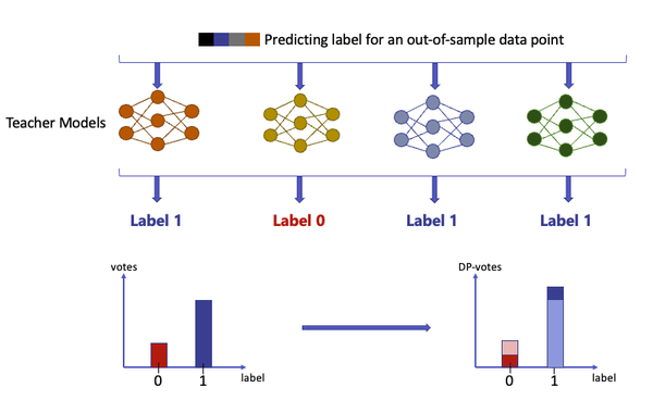
Figure 7-2. Differentially private classification with PATE framework.
PATE, as described so far, can be used as a differentially private API. Differential privacy guarantees come from the fact that each label is predicted by the noisy aggregation mechanism. Notice that the addition or removal of an individual from the dataset would affect the output of only one of the teacher models. This means that, by applying a differential privacy mechanism to the counts of votes, we guarantee that the output of the prediction is differentially private.
Using PATE to train a differentially private model
The PATE framework is easy to implement and provides differential privacy during inference for any machine learning technique you apply it to. However, there is one significant limitation: each prediction made spends part of the total privacy budget. This means that there is a limit to how many times this model can be used to make predictions.
This problem can be solved by creating a student model that learns from the teacher models predictions. Since the student model is post-processing the differentially private data, the final student model is differentially private, and can be used as many times as desired without affecting the privacy budget.
Let’s assume the availability of a private labelled dataset and a public unlabelled dataset. The student model is trained as follows:
-
Label the public unlabelled dataset utilizing PATE framework, trained on the private labelled dataset.
-
Use the dataset labelled in the previous step to train a student model.
The following diagram shows this process: the public unlabeled data is sent to the teacher models, which generate a DP histogram of labels. From this histogram, a label is added to the data and sent to train the student model.
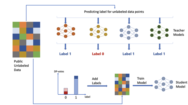
Figure 7-3. Differentially private learning with PATE framework for classification.
The student model can be deployed to respond to any prediction queries from end users. Most importantly, the private data and teacher models can safely be discarded. Notice that the overall privacy budget is now fixed to a constant value once the student has completed its training. An additional important characteristic of the student model is that an adversary with access to the student’s model weights and parameters could in the worst-case only recover the labels on which the student model was trained. The labels in this case are all differentially private, which is guaranteed by the noisy aggregation mechanism.
In this chapter, you have learned about approaches for building differentially private machine learning models. This often involves modifying existing models, in particular, transforming linear regression and stochastic gradient descent algorithms to be differentially private. Another approach, highlighted in this chapter, is PATE, a general framework for transforming any learning task into a differentially private learning task. On the implementation side, you’ve learned about Opacus as a tool for implementing DP-SGD and PATE.
Now that you are familiar with the basics of DP machine learning, you are ready to learn about the nuances of implementing DP machine learning models in the real world. You will need to take a variety of factors into account during the model training process. In the next chapter, you will learn about budget composition, batching and hyperparameter tuning. The next chapter also provides several code examples for the techniques introduced in this chapter. By the end of next chapter, you will be able to train your own differentially private learning model.
Exercises
-
a. Given the function
-
How does the speed of the program change with changes in gamma?
-
-
a. Starting with the mean squared error as for linear regression, calculate the gradient.
-
Generate linear data with noise added to it (via numpy or a similar package). Write code that uses the gradient you just calculated to find the minimum of the error function.
-
-
Implement a DP version of simple linear regression using the Theil-Sen mechanism. How do your model parameters compare to a non-DP implementation?
1 R. Shokri, M. Stronati, C. Song, and V. Shmatikov, “Membership Inference Attacks against Machine Learning Models.” arXiv, Mar. 31, 2017. Accessed: Jun. 09, 2023. Available: http://arxiv.org/abs/1610.05820
2 For more information on attacks, see Ch. 10 (Chapter 10)