Chapter 8: Self-Attention for Image Generation
You may have heard about some popular Natural Language Processing (NLP) models, such as the Transformer, BERT, or GPT-3. They all have one thing in common – they all use an architecture known as a transformer that is made up of self-attention modules.
Self-attention is gaining widespread adoption in computer vision, including classification tasks, which makes it an important topic to master. As we will learn in this chapter, self-attention helps us to capture important features in the image without using deep layers for large effective receptive fields. StyleGAN is great for generating faces, but it will struggle to generate images from ImageNet.
In a way, faces are easy to generate, as eyes, noses, and lips all have similar shapes and are in similar positions across various faces. In contrast, the 1,000 classes of ImageNet contain varied objects (dogs, trucks, fish, and pillows, for instance) and backgrounds. Therefore, the discriminator must be more effective at capturing the distinct features of various objects. This is where self-attention comes into play. Using that, with conditional batch normalization and spectral normalization, we will implement a Self-Attention GAN (SAGAN) to generate images based on given class labels.
After that, we will use the SAGAN as a base to create a BigGAN. We will add orthogonal regularization and change the method of doing class embedding. BigGANs can generate high-definition images without using ProGAN-like architecture, and they are considered to be state-of-the-art models in class labels conditioning image generation.
We will cover the following topics in this chapter:
- Spectral normalization
- Self-attention modules
- Building a SAGAN
- Implementing BigGAN
Technical requirements
The Jupyter notebooks can be found here (https://github.com/PacktPublishing/Hands-On-Image-Generation-with-TensorFlow-2.0/tree/master/Chapter08):
- ch8_sagan.ipynb
- ch8_big_gan.ipynb
Spectral normalization
Spectral normalization is an important method to stabilize GAN training and it has been used in a lot of recent state-of-the-art GANs. Unlike batch normalization or other normalization methods that normalize the activation, spectral normalization normalizes the weights instead. The aim of spectral normalization is to limit the growth of the weights, so the networks adhere to the 1-Lipschitz constraint. This has proved effective in stabilizing GAN training, as we learned in Chapter 3, Generative Adversarial Network.
We will revise WGANs to give us a better understanding of the idea behind spectral normalization. The WGAN discriminator (also known as the critic) needs to keep its prediction to small numbers to meet the 1-Lipschtiz constraint. WGANs do this by naively clipping the weights to the range of [-0.01, 0.01].
This is not a reliable method as we need to fine-tune the clipping range, which is a hyperparameter. It would be nice if there was a systematic way to enforce the 1-Lipschitz constraint without the use of hyperparameters, and spectral normalization is the tool we need for that. In essence, spectral normalization normalizes the weights by dividing by their spectral norms.
Understanding spectral norm
We will go over some linear algebra to roughly explain what spectral norm is. You may have learned about eigenvalues and eigenvectors in matrix theory with the following equation:
Here A is a square matrix, v is the eigenvector, and the lambda is its eigenvalue.
We'll try to understand the terms using a simple example. Let's say that v is a vector of position (x, y) and A is a linear transformation as follows:

If we multiply A with v, we'll get a new position with a change of direction as follows:

Eigenvectors are vectors that do not change their directions when A is applied to them. Instead, they are only scaled by the scalar eigenvalues denoted as lambda. There can be multiple eigenvector-eigenvalue pairs. The square root of the largest eigenvalue is the spectral norm of the matrix. For a non-square matrix, we will need to use a mathematical algorithm such as singular value decomposition (SVD) to calculate the eigenvalues, which can be computationally costly.
Therefore, a power iteration method is employed to speed up the calculation and make it feasible for neural network training. Let's jump in to implement spectral normalization as a weight constraint in TensorFlow.
Implementing spectral normalization
The mathematic algorithm of spectral normalization as given by T. Miyato et al., 2018, in the Spectral Normalization For Generative Adversarial Networks paper may appear complex. However, as usual, the software implementation is simpler than what the mathematics looks.
The following are the steps to perform spectral normalization:
- The weights in the convolutional layer form a 4-dimensional-tensor, so the first step is to reshape it into a 2D matrix of W, where we keep the last dimension of the weight. Now the weight has the shape (H×W, C).
- Initialize a vector u with N(0,1).
- In a for loop, calculate the following:
a) Calculate V = (WT) U with matrix transpose and matrix multiplication.
b) Normalize V with its L2 norm, that is, V = V/||V||2.
c) Calculate U = WV.
d) Normalize U with its L2 norm, that is, U = U/||U||2.
- Calculate the spectral norm as UTW V.
- Finally, divide the weights by the spectral norm.
The full code is as follows:
class SpectralNorm(tf.keras.constraints.Constraint):
def __init__(self, n_iter=5):
self.n_iter = n_iter
def call(self, input_weights):
w = tf.reshape(input_weights, (-1, input_weights.shape[-1]))
u = tf.random.normal((w.shape[0], 1))
for _ in range(self.n_iter):
v = tf.matmul(w, u, transpose_a=True)
v /= tf.norm(v)
u = tf.matmul(w, v)
u /= tf.norm(u)
spec_norm = tf.matmul(u, tf.matmul(w, v), transpose_a=True)
return input_weights/spec_norm
The number of iterations is a hyperparameter, and I found 5 to be sufficient. Spectral normalization can also be implemented to have a variable to remember the vector u rather than starting from random values. This should reduce the number of iterations to 1. We can now apply spectral normalization by using it as a kernel constraint when defining layers, as in Conv2D(3, 1, kernel_constraint=SpectralNorm()).
Self-attention modules
Self-attention modules became popular with the introduction of an NLP model known as the Transformer. In NLP applications such as language translation, the model often needs to read sentences word by word to understand them before producing the output. The neural network used prior to the advent of the Transformer was some variant on the recurrent neural network (RNN), such as long short-term memory (LSTM). The RNN has internal states to remember words as it reads a sentence.
One drawback of that is that when the number of words increases, the gradients for the first words vanish. That is to say, the words at start of the sentence become less important gradually as the RNN reads more words.
The Transformer does things differently. It reads all the words at once and weights the importance of each individual word. Therefore, more attention is given to words that are more important, and hence the name attention. Self-attention is a cornerstone of state-of-the-art NLP models such as BERT and GPT-3. However, NLP is not in the scope of this book. We will now look at the details of how self-attention works in CNN.
Self-attention for computer vision
CNNs are mainly made up of convolutional layers. For a convolutional layer with a kernel size of 3×3, it will only look at 3×3=9 features in the input activation to compute each output feature. It will not look at pixels outside of this range. To capture the pixels outside of this range, we could increase the kernel size slightly to, say, 5×5 or 7×7, but that is still small compared to the feature map size.
We will have to move down one network layer for the convolutional kernel's receptive field to be large enough to capture what we want. As with RNNs, the relative importance of the input features fades as we move down through the network layers. Thus, we can use self-attention to look at every pixel in the feature map and work on what we should pay attention to.
We will now look at how the self-attention mechanism works. The first step of self-attention is to project each input feature into three vectors known as the key, query, and value. We don't see these terms a lot in computer vision literature, but I thought it would be good to teach you about them so that you can better understand general self-attention-, Transformer-, or NLP-related literature. The following figure illustrates how attention maps are generated from a query:

Figure 8.1 – Illustration of an attention map. (Source: H. Zhang et al., 2019, "Self-Attention Generative Adversarial Networks," https://arxiv.org/abs/1805.08318)
On the left is an image with queries marked with dots. The next five images show the attention maps given by the queries. The first attention map on the top queries one eye of the rabbit; the attention map has more white (indicating areas of high importance) around both the eyes and close to complete darkness (for low importance) in other areas.
Now, we'll now go over the technical terms of key, query, and value one by one:
- A value is a representation of the input features. We don't want the self-attention module to look at every single pixel as this will be too computationally expensive and unnecessary. Instead, we are more interested in the local regions of the input activation. Therefore, the value has reduced dimensions from the input features, both in terms of the activation map size (for example, it may be downsampled to have smaller height and width) and the number of channels. For convolutional layer activations, the channel number is reduced by using a 1x1 convolution, and the spatial size is reduced by max-pooling or average pooling.
- Keys and queries are used to compute the importance of the features of the self-attention map. To calculate an output feature at location x, we take query at location x and compare it with the key at all locations. To illustrate more on this, let's say we have an image of a portrait.
When the network is processing one eye of the portrait, it will take its query, which has a semantic meaning of eye, and check that with the keys of other areas of the portrait. If one of the other areas' keys is eye, then we know we have found the other eye, and it certainly is something we want to pay attention to so that we can match the eye color.
To put that into an equation, for feature 0, we calculate a vector of q0 × k0, q0 × k1, q0 × k2 and so on to q0 × kN-1. The vectors are then normalized using softmax so they all sum up to 1.0, which is our attention score. This is used as a weight to perform element-wise multiplication of the value, to give the attention outputs.
The SAGAN self-attention module is based on the non-local block (X. Wang et al., 2018, Non-local Neural Networks, https://arxiv.org/abs/1711.07971), which was originally designed for video classification. The authors experimented with different ways of implementing self-attention before settling on the current architecture. The following diagram shows the attention module in SAGAN, where theta θ, phi φ, and g correspond to key, query, and value:

Figure 8.2 – Self-attention module architecture in SAGAN
Most computation in deep learning is vectorized for speed performance, and it is no different for self-attention. If we ignore the batch dimension for simplicity, the activations after 1×1 convolution will have a shape of (H, W, C). The first step is to reshape it into a 2D matrix with a shape of (H×W, C) and use the matrix multiplication between θ and φ to calculate the attention map. In the self-attention module used in SAGAN, there is another 1×1 convolution that is used to restore the channel number to the input channel, followed by scaling with learnable parameters. Furthermore, this is made into a residual block.
Implementing a self-attention module
We will first define all the 1×1 convolutional layers and weights in the custom layer's build(). Please note that we use a spectral normalization function as the kernel constraint for the convolutional layers as follows:
class SelfAttention(Layer):
def __init__(self):
super(SelfAttention, self).__init__()
def build(self, input_shape):
n, h, w, c = input_shape
self.n_feats = h * w
self.conv_theta = Conv2D(c//8, 1, padding='same', kernel_constraint=SpectralNorm(), name='Conv_Theta')
self.conv_phi = Conv2D(c//8, 1, padding='same', kernel_constraint=SpectralNorm(), name='Conv_Phi')
self.conv_g = Conv2D(c//2, 1, padding='same', kernel_constraint=SpectralNorm(), name='Conv_G')
self.conv_attn_g = Conv2D(c, 1, padding='same', kernel_constraint=SpectralNorm(), name='Conv_AttnG')
self.sigma = self.add_weight(shape=[1], initializer='zeros', trainable=True, name='sigma')
There are a few things to note here:
- The internal activation can have reduced dimensions to make the computation run faster. The reduced numbers were obtained by the SAGAN authors by experimentation.
- After every convolution layer, the activation (H, W, C) is reshaped into two- dimensional matrix with the shape (HW, C). We can then use matrix multiplication on the matrices.
The following is the call() function of the layer to perform the self-attention operations. We will first calculate theta, phi, and g:
def call(self, x):
n, h, w, c = x.shape
theta = self.conv_theta(x)
theta = tf.reshape(theta, (-1, self.n_feats, theta.shape[-1]))
phi = self.conv_phi(x)
phi = tf.nn.max_pool2d(phi, ksize=2, strides=2, padding='VALID')
phi = tf.reshape(phi, (-1, self.n_feats//4, phi.shape[-1]))
g = self.conv_g(x)
g = tf.nn.max_pool2d(g, ksize=2, strides=2, padding='VALID')
g = tf.reshape(g, (-1, self.n_feats//4, g.shape[-1]))
We will then calculate the attention map as follows:
attn = tf.matmul(theta, phi, transpose_b=True) attn = tf.nn.softmax(attn)
Finally, we multiply attention map with the query g and proceed to produce the final output:
attn_g = tf.matmul(attn, g)
attn_g = tf.reshape(attn_g, (-1, h, w, attn_g.shape[-1]))
attn_g = self.conv_attn_g(attn_g)
output = x + self.sigma * attn_g
return output
With the spectral normalization and self-attention layers written, we can now use them to build a SAGAN.
Building a SAGAN
The SAGAN has a simple architecture that looks like DCGAN's. However, it is a class-conditional GAN that uses class labels to both generate and discriminate between images. In the following figure, each image on each row is generated from different class labels:

Figure 8.3 – Images generated by a SAGAN by using different class labels. (Source: A. Brock et al., 2018, "Large Scale GAN Training for High Fidelity Natural Image Synthesis," https://arxiv.org/abs/1809.11096)
In this example, we will use the CIFAR10 dataset, which contains 10 classes of images with a resolution of 32x32. We will deal with the conditioning part later. Now, let's first complete the simplest part – the generator.
Building a SAGAN generator
At a high level, the SAGAN generator doesn't look very different from other GAN generators: it takes noise as input and goes through a dense layer, followed by multiple levels of upsampling and convolution blocks, to achieve the target image resolution. We start with 4×4 resolution and use three upsampling blocks to reach the final resolution of 32×32, as follows:
def build_generator(z_dim, n_class):
DIM = 64
z = layers.Input(shape=(z_dim))
labels = layers.Input(shape=(1), dtype='int32')
x = Dense(4*4*4*DIM)(z)
x = layers.Reshape((4, 4, 4*DIM))(x)
x = layers.UpSampling2D((2,2))(x)
x = Resblock(4*DIM, n_class)(x, labels)
x = layers.UpSampling2D((2,2))(x)
x = Resblock(2*DIM, n_class)(x, labels)
x = SelfAttention()(x)
x = layers.UpSampling2D((2,2))(x)
x = Resblock(DIM, n_class)(x, labels)
output_image = tanh(Conv2D(3, 3, padding='same')(x))
return Model([z, labels], output_image, name='generator')
Despite using different activation dimensions within the self-attention module, its output has the same shape as the input. Thus, this can be inserted anywhere after a convolutional layer. However, it may be overkill to put it at 4×4 resolution when the kernel size is 3×3. So, the self-attention layer is inserted only once in the SAGAN generator at a higher spatial resolution stage to make the most out of the self-attention layer. The same goes for the discriminator, where the self-attention layer is placed at the lower layer when the spatial resolution is higher.
That's all for the generator, if we're doing unconditional image generation. We will need to feed the class labels into the generator so it can create images from the given classes. At the beginning of Chapter 4, Image-to-Image Translation, we learned about some common ways of conditioning on labels, but the SAGAN uses a more advanced way; that is, it encodes the class label into learnable parameters in batch normalization. We introduced conditional batch normalization in Chapter 5, Style Transfer, and we will now implement it for the SAGAN.
Conditional batch normalization
Throughout much of this book, we have been complaining about the drawback of using batch normalization in GANs. In CIFAR10, there are 10 classes: 6 of them are animals (bird, cat, deer, dog, frog, and horse) and 4 of them are vehicles (airplane, automobile, ship, and truck). Obviously, they look very different –the vehicles tend to have hard and straight edges, while the animals tend to have curvier edges and softer textures.
As we have learned regarding style transfer, the activation statistics dictate the image style. Therefore, mixing the batch statistics can create images that look a bit like an animal and a bit like a vehicle – for example, a car-shaped cat. This is because batch normalization uses only one gamma and one beta for an entire batch that's made up of different classes. The problem is resolved if we have a gamma and a beta for each of the styles (classes), and that is exactly what conditional batch normalization is about. It has one gamma and one beta for each class, so there are 10 betas and 10 gammas per layer for the 10 classes in CIFAR10.
We can now construct the variables required by the conditional batch normalization as follows:
- A gamma and a beta with a shape of (10, C), where C is the activation channel number.
- A moving mean and variance with a shape of (1, 1, 1, C). In training, the mean and variance are calculated from a minibatch. During inference, we use the moving averaged values accumulated in training. They are shaped so that the arithmetic operation is broadcast to the N, H, and W dimensions.
The following is the code for conditional batch normalization:
class ConditionBatchNorm(Layer):
def build(self, input_shape):
self.input_size = input_shape
n, h, w, c = input_shape
self.gamma = self.add_weight( shape=[self.n_class, c], initializer='ones', trainable=True, name='gamma')
self.beta = self.add_weight( shape=[self.n_class, c], initializer='zeros', trainable=True, name='beta')
self.moving_mean = self.add_weight(shape=[1, 1, 1, c], initializer='zeros', trainable=False, name='moving_mean')
self.moving_var = self.add_weight(shape=[1, 1, 1, c], initializer='ones',
trainable=False, name='moving_var')
When we run the conditional batch normalization, we retrieve the correct beta and gamma for the labels. This is done using tf.gather(self.beta, labels), which is conceptually equivalent to beta = self.beta[labels], as follows:
def call(self, x, labels, training=False):
beta = tf.gather(self.beta, labels)
beta = tf.expand_dims(beta, 1)
gamma = tf.gather(self.gamma, labels)
gamma = tf.expand_dims(gamma, 1)
Apart from that, the rest of the code is identical to batch normalization. Now, we can place the conditional batch normalization in the residual block for the generator:
class Resblock(Layer):
def build(self, input_shape):
input_filter = input_shape[-1]
self.conv_1 = Conv2D(self.filters, 3, padding='same', name='conv2d_1')
self.conv_2 = Conv2D(self.filters, 3, padding='same', name='conv2d_2')
self.cbn_1 = ConditionBatchNorm(self.n_class)
self.cbn_2 = ConditionBatchNorm(self.n_class)
self.learned_skip = False
if self.filters != input_filter:
self.learned_skip = True
self.conv_3 = Conv2D(self.filters, 1, padding='same', name='conv2d_3')
self.cbn_3 = ConditionBatchNorm(self.n_class)
The following is the runtime code for the forward pass of conditional batch normalization:
def call(self, input_tensor, labels):
x = self.conv_1(input_tensor)
x = self.cbn_1(x, labels)
x = tf.nn.leaky_relu(x, 0.2)
x = self.conv_2(x)
x = self.cbn_2(x, labels)
x = tf.nn.leaky_relu(x, 0.2)
if self.learned_skip:
skip = self.conv_3(input_tensor)
skip = self.cbn_3(skip, labels)
skip = tf.nn.leaky_relu(skip, 0.2)
else:
skip = input_tensor
output = skip + x
return output
The residual block for the discriminator looks similar to the one for the generator but with a couple of differences, as listed here:
- There is no normalization.
- Downsampling happens inside the residual block with average pooling.
Therefore, we won't be showing the code for the discriminator's residual block. We can now proceed to the final building block – the discriminator.
Building the discriminator
The discriminator uses the self-attention layer as well, and it is placed near the input layers to capture the large activation map. As it is a conditional GAN, we will also use the label in the discriminator to make sure that the generator is producing the correct images matching the classes. The general approach to incorporating label information is to first project the label into the embedding space and then use the embedding at either the input layer or any internal layer.
There are two common methods of merging the embedding with the activation – concatenation and element-wise multiplication. The SAGAN uses architecture that's similar to the projection model by T. Miyato and M. Koyama's cGANs with Projection Discriminator, as shown at the bottom right of the following figure:
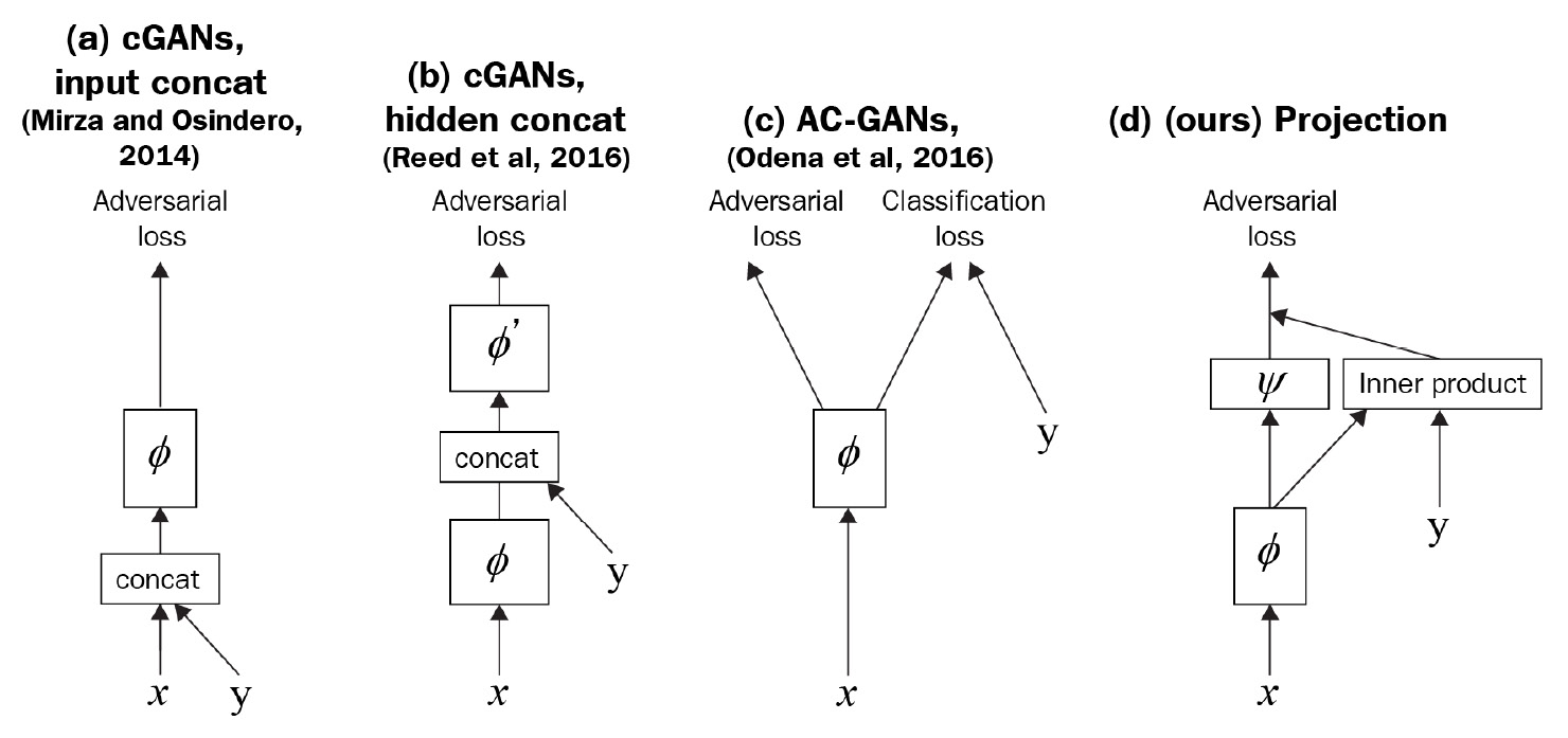
Figure 8.4 – Comparison of several common ways of incorporating labels as conditions in a discriminator. (d) is the one used in the SAGAN. (Redrawn from T. Miyato and M. Koyama's, 2018 "cGANs with Projection Discriminator," https://arxiv.org/abs/1802.05637)
The label is first projected into embedding space, and then we perform element-wise multiplication with activation just before the dense layer (ψ in the diagram). The result then adds to the dense layer output to give the final prediction as follows:
def build_discriminator(n_class):
DIM = 64
input_image = Input(shape=IMAGE_SHAPE)
input_labels = Input(shape=(1))
embedding = Embedding(n_class, 4*DIM)(input_labels)
embedding = Flatten()(embedding)
x = ResblockDown(DIM)(input_image) # 16
x = SelfAttention()(x)
x = ResblockDown(2*DIM)(x) # 8
x = ResblockDown(4*DIM)(x) # 4
x = ResblockDown(4*DIM, False)(x) # 4
x = tf.reduce_sum(x, (1, 2))
embedded_x = tf.reduce_sum(x * embedding, axis=1, keepdims=True)
output = Dense(1)(x)
output += embedded_x
return Model([input_image, input_labels], output, name='discriminator')
With the models defined, we can now train the SAGAN.
Training the SAGAN
We will use the standard GAN training pipeline. The loss function is hinge loss and we will use the Adam optimizer. Different initial learning rates are used for the generator (1e-4) and discriminator (4e-4). As CIFAR10 has small images of size 32×32, the training is relatively stable and quick. The original SAGAN was designed for an image resolution of 128×128, but this resolution is still small compared to other training sets that we have used. In the next section, we will look at some improvements made to the SAGAN for training on bigger datasets with bigger image sizes.
Implementing BigGAN
The BigGAN is an improved version of the SAGAN. The BigGAN ups the image resolution significantly from 128×128 to 512×512, and it does it without progressive growth of layers! The following are some sample images generated by BigGAN:
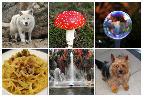
Figure 8.5 – Class-conditioned samples generated by BigGAN at 512x512 (Source: A. Brock et al., 2018, "Large Scale GAN Training for High Fidelity Natural Image Synthesis," https://arxiv.org/abs/1809.11096)
BigGAN is considered the state-of-the-art class-conditional GAN. We'll now look into the changes and modify the SAGAN code to make ourselves a BigGAN.
Scaling GANs
Older GANs tend to use small batch sizes as that would produce better-quality images. Now we know that the quality problem was caused by the batch statistics used in batch normalization, and this is addressed by using other normalization techniques. Still, the batch size has remained small as it is physically limited by GPU memory constraints.
However, being part of Google has its perks: the DeepMind team, who created the BigGAN, had all the resources they needed. Through experimentation, they found that scaling up GANs helps in producing better results. In BigGAN training, the batch size used was eight times that of the SAGAN; the convolutional channel numbers are also 50% higher. This is where the name BigGAN came from: bigger proved to be better.
As a matter of fact, the bulking up of the SAGAN is the main contributor to BigGAN's superior performance, as summarized in the following table:

Figure 8.6 – Improvement in Frechet Inception Distance (FID) and Inception Score (IS) by adding features to the SAGAN baseline. The Configurations column shows the features added to the configuration in the previous row. The numbers in brackets show the improvement on the preceding row
The table shows the BigGAN's performance when trained on ImageNet. The Frechet Inception Distance (FID) measures the class variety (the lower the better), while the Inception Score (IS) indicates the image quality (the higher the better). On the left is the configuration of the network, starting with the SAGAN baseline and adding new features row by row. We can see that the biggest improvement came from increasing the batch size. This makes sense for improving the FID, as a batch size of 2,048 is larger than the class size of 1,000, making the GAN less likely to overfit to the small number of classes.
Increasing the channel size also resulted in significant improvement. The other three features add only a small improvement. Therefore, if you don't have multiple GPUs that can fit a large network and batch size, then you should stick to the SAGAN. If you do have such GPUs or just want to know about the feature upgrades, then let's crack on!
Skipping latent vectors
Traditionally, the latent vector z goes into the first dense layer of the generator, followed by a sequence of convolutional and upsampling layers. Although the StyleGAN also has a latent vector that goes only to the first layer of its generator, it has another source of random noise that goes into every resolution of the activation map. This allows the control of style at different resolution levels.
By merging the two ideas, the BigGAN split the latent vector into chunks, where each of them goes to different residual blocks in the generator. Later, we will see how that concatenates with the class label for conditional batch normalization. In addition to the default BigGAN, there is another configuration known as BigGAN-deep that is four times deeper. The following diagram shows their difference in concatenating labels and input noise. We will implement the BigGAN on the left:
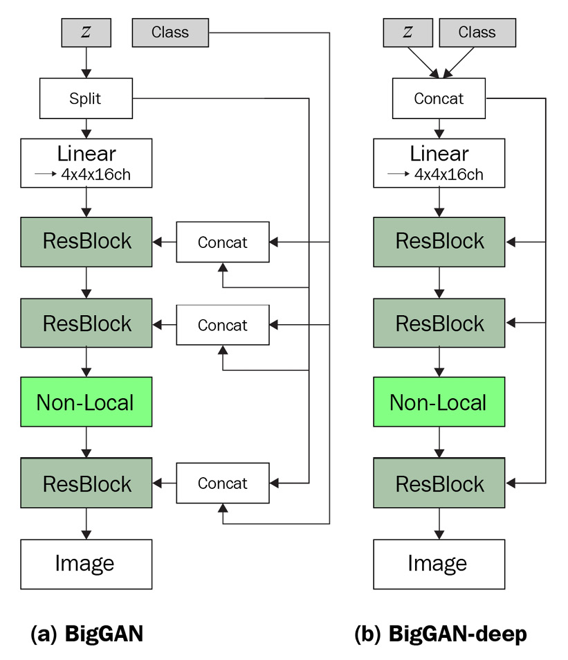
Figure 8.7 – Two configurations of the generator (Redrawn from A. Brock et al., 2018, "Large Scale GAN Training for High Fidelity Natural Image Synthesis," https://arxiv.org/abs/1809.11096)
We will now look at how BigGAN reduces the size of the embedding in conditional batch normalization.
Shared class embedding
In the SAGAN's conditional batch normalization, there is a matrix of the shape [class number, channel number] for each beta and gamma in every layer. When the number of classes and channels increases, the weight size goes up rapidly too. When trained on the 1,000-class ImageNet with 1,024-channel convolutional layers, this will create over 1 million variables in one normalization layer alone!
Therefore, instead of having a weight matrix of 1,000×1,024, the BigGAN first projects the class into an embedding of smaller dimensions, for example, 128, that is shared across all layers. Within the conditional batch normalization, dense layers are used to map the class embedding and noise into betas and gammas.
The following code snippet shows the first two layers in the generator:
z_input = layers.Input(shape=(z_dim))
z = tf.split(z_input, 4, axis=1)
labels = layers.Input(shape=(1), dtype='int32')
y = Embedding(n_class, y_dim)(tf.squeeze(labels, [1]))
x = Dense(4*4*4*DIM, **g_kernel_cfg)(z[0])
x = layers.Reshape((4, 4, 4*DIM))(x)
x = layers.UpSampling2D((2,2))(x)
y_z = tf.concat((y, z[1]), axis=-1)
x = Resblock(4*DIM, n_class)(x, y_z)
The latent vector with dimensions of 128 is first split into four equal parts, for the dense layer and the residual blocks at three resolutions. The label is projected into a shared embedding that concatenates with the z chunk and goes into residual blocks. The residual blocks are unchanged from the SAGAN, but we'll make some small modifications to the conditional batch normalization in the following code. Instead of declaring variables for gamma and beta, we now generate from class labels via dense layers. As usual, we will first define the required layers in build() as shown here:
class ConditionBatchNorm(Layer):
def build(self, input_shape):
c = input_shape[-1]
self.dense_beta = Dense(c, **g_kernel_cfg,)
self.dense_gamma = Dense(c, **g_kernel_cfg,)
self.moving_mean = self.add_weight(shape=[1, 1, 1, c], initializer='zeros', trainable=False, name='moving_mean')
self.moving_var = self.add_weight(shape=[1, 1, 1, c], initializer='ones', trainable=False, name='moving_var')
At runtime, we will use dense layers to generate beta and gamma from the shared embedding. Then, they will be used like normal batch normalization. The code snippet for the dense layer parts are shown here:
def call(self, x, z_y, training=False):
beta = self.dense_beta(z_y)
gamma = self.dense_gamma(z_y)
for _ in range(2):
beta = tf.expand_dims(beta, 1)
gamma = tf.expand_dims(gamma, 1)
We added dense layers to predict beta and gamma from the latent vector and label embedding. That replaces the large weight variables.
Orthogonal regularization
Orthogonality is used extensively in the BigGAN to initialize weights and as a weight regularizer. A matrix is said to be orthogonal if multiplication with its transpose will produce an identity matrix. An identity matrix is a matrix with one in the diagonal elements and zero in all other places. Orthogonality is a good property because the norm of a matrix doesn't change if it is multiplied by an orthogonal matrix.
In a deep neural network, the repeated matrix multiplication can result in exploding or vanishing gradients. Therefore, maintaining orthogonality can improve training. The equation for original orthogonal regularization is as follows:

Here W is the weight reshaped as a matrix and beta is a hyperparameter. As this regularization was found to be limiting, the BigGAN uses a different variant:

In this variant, (1 – I) removes the diagonal elements, which are dot products of the filters. This removes the constraint on the filter's norm and aims to minimize the pairwise cosine similarity between the filters.
Orthogonality is closely related to spectral normalization, and both can co-exist in a network. We implemented spectral normalization as a kernel constraint, where the weights are modified directly. Weight regularization calculates the loss from the weights and adds the loss to other losses for backpropagation, hence regularizing the weights in an indirect way. The following code shows how to write a custom regularizer in TensorFlow:
class OrthogonalReguralizer( tf.keras.regularizers.Regularizer):
def __init__(self, beta=1e-4):
self.beta = beta
def __call__(self, input_tensor):
c = input_tensor.shape[-1]
w = tf.reshape(input_tensor, (-1, c))
ortho_loss = tf.matmul(w, w, transpose_a=True) * (1 -tf.eye(c))
return self.beta * tf.norm(ortho_loss)
def get_config(self):
return {'beta': self.beta}
We can then assign the kernel initializer, kernel constraint, and kernel regularizer to the convolution and dense layers. However, adding them to each of the layers can make the code look long and cluttered. To avoid this, we can put them into a dictionary and pass them as keyword arguments (kwargs) into the Keras layers as follows:
g_kernel_cfg={
'kernel_initializer' : tf.keras.initializers.Orthogonal(),
'kernel_constraint' : SpectralNorm(),
'kernel_regularizer' : OrthogonalReguralizer()
}
Conv2D(1, 1, padding='same', **g_kernel_cfg)
As we mentioned earlier, orthogonal regularization has the smallest effect in improving image quality. The beta value of 1e-4 was obtained numerically, and you might need to tune it for your dataset.
Summary
In this chapter, we learned about an important network architecture known as self-attention. The effectiveness of the convolutional layer is limited by its receptive field, and self-attention helps to capture important features including activations that are spatially-distanced from conventional convolutional layers. We have learned how to write a custom layer to insert into a SAGAN. The SAGAN is a state-of-the-art class-conditional GAN. We also implemented conditional batch normalization to learn different learnable parameters specific to each class. Finally, we looked at the bulked-up version of the SAGAN known as the BigGAN, which trumps SAGAN's performance significantly in terms of both image resolution and class variation.
We have now learned about most, if not all, of the important GANs for image generation. In recent years, two major components have gained popularity in the GAN world – they are AdaIN for the StyleGAN as covered in Chapter 7, High Fidelity Face Generation and self-attention for the SAGAN. The Transformer is based on self-attention and has revolutionized NLP, and it's starting to make its way into computer vision. Therefore, it is now a good time to learn about attention-based generative models as this may be how future GANs look. In the next chapter, we will use what we learned about image generation at the end of this chapter to generate a deepfake video.