Chapter 3: Entanglement and Quantum Teleportation

In this chapter, we will cover the fundamentals of entanglement, and how it came to be referred to as spooky action at a distance. Entanglement plays a crucial role in quantum information processing, so it is imperative to have a chapter dedicated to entanglement.

After covering the fundamentals of entanglement, the chapter will discuss the Bell theorem and the tests of entanglement. Finally, the chapter will discuss one of the applications of entanglement, namely, quantum teleportation.

In this chapter, we will cover the following main topics:

• Exploring the history of quantum entanglement
• Understanding the Bell theorem and CHSH inequality
• Understanding composite systems and entanglement
• Understanding the CNOT gate – the entangling gate
• Understanding Bell states
• Understanding the entanglement of more than two quantum states
• Understanding entanglement as a resource – quantum teleportation

Technical requirements

The requirements for this chapter are the following:

• A basic understanding of the Python programming language
• Navigation of Google's Colab environment
• Elementary (post-secondary) mathematics knowledge

The GitHub link for this chapter can be found here: https://github.com/PacktPublishing/Hands-On-Quantum-Information-Processing-with-Python/tree/master/Chapter03.

In the next section, we will cover the brief history of quantum entanglement.

Exploring the history of quantum entanglement

In our day-to-day lives, we are quite familiar with correlations of various affairs. At a sub-atomic level though, correlations of quantum particles go beyond our day-to-day experience. These quantum correlations are referred to as quantum entanglement. The term entanglement was coined by a German physicist, Erwin Schrödinger, using the German word Verschränkung, which he translated to mean entanglement.

In essence, quantum entanglement occurs when two quantum particles that have interacted remain a single, indivisible system, even if such quantum systems are separated by an arbitrarily long distance. This way, the quantum particles remain inter-dependent, and hence correlated. This means that for these entangled particles, if an action is performed on one particle, the second particle will also be affected by that action, and this influence occurs instantaneously.

Albert Einstein, who was one of the greatest scientists of the 20th century, was a firm critic of quantum entanglement. He referred to entanglement as spooky action at a distance because quantum entanglement suggests an instantaneous correlation between two quantum particles that are separated by an arbitrarily long distance.

In 1935, Einstein, together with his colleagues Boris Podolsky and Nathan Rosen, presented a very serious critique of quantum entanglement. This critique was presented in the form of a thought experiment, which would later be referred to as the EPR paradox (also referred to as the Einstein-Podolsky-Rosen paradox).

Through the formulation of the EPR paradox, Einstein, Podolsky, and Rosen used the concept of quantum entanglement to demonstrate that quantum mechanics cannot provide a complete description of reality and that it should be supplemented by additional parameters, the hidden variables.

The EPR paradox can be explained as follows. Consider two correlated quantum particles, Alice and Bob (thus, Alice and Bob are entangled). At first, Alice and Bob are allowed to interact. Then, Alice and Bob are separated such that they are so far apart that it would be impossible for them to communicate with one another.

Since Alice and Bob are entangled, the operations performed on one will also affect the other. Therefore, for instance, if measurement is performed on Alice, the influence of that correlation would be instantaneously reflected by Bob. The paradox in this (in the EPR paradox) is that this would imply that this influence would travel faster than the speed of light, and this is in direct conflict with the known fact that nothing travels faster than light.

The EPR paradox provided a serious challenge to quantum mechanics for nearly three decades. However, in 1964, the physicist John Bell proved that the interpretation given in the EPR paradox is inconsistent with quantum mechanics. This proof later came to be known as the Bell theorem, and will be discussed later in this chapter.

Like Einstein, Podolsky, and Rosen, Bell used a thought experiment in order to develop his theorem. However, since his theorem made testable predictions, these predictions were later tested experimentally. The first experiment was performed by John Clauser and Stuart Freedman in 1972.

Another experiment was conducted by Edward Fry and Randall Thompson in 1976. Furthermore, in the 1980s, Alain Aspect performed an entanglement-based experiment. Finally, in the late 1990s, Anton Zeilinger performed a set of experiments that firmly established the reality of quantum mechanics and hence provided a serious blow to the interpretation given in the EPR paradox.

Having provided a brief history of the concept of quantum entanglement, it is now imperative to further explore this concept. This exploration will be done in the next section, where the Bell theorem and CHSH inequality will be covered.

Understanding the Bell theorem and CHSH inequality

As already stated in the previous section, Bell's theorem renders the quantum mechanical interpretation used in the EPR paradox obsolete. This philosophical interpretation is known as local realism. The realism in this case posits that objects exist even when they are not observed/measured. For instance, the moon does exist regardless of whether you are looking at it. On the other hand, local in local realism posits that an event at one point cannot instantaneously have an effect at another point. This interpretation is also known as the hidden variables interpretation of quantum mechanics.

In order to address the hidden variables argument, Bell came up with a thought experiment that would test the validity of this interpretation. This thought experiment was later reformulated by the physicist David Bohm, who used the spin properties of quantum mechanical systems such as electrons.

Consider two quantum variables, each with a spin angular momentum. Now, consider the random variables A1α A2α to be the outcomes of the spin measurements made along the axes α = x, y, and z, and taking the values -1 or 1. Then, if the correlations from these measurements are not quantum mechanical (there is no quantum entanglement), and if the aforementioned random variables are anti-correlated, then for probability p (as predicted by the hidden variables interpretation), we have the following:

The inequality in the given equation is known as the Bell theorem, or Bell's inequality. Any quantum mechanical correlation, quantum entanglement, violates Bell's inequality.

Bell's inequality was later generalized by Clauser, Horne, Shimony, and Holt, in what would later be known as the CHSH inequality. The CHSH inequality is briefly summarized as follows.

Consider two quantum particles, Alice and Bob, and the detector measurement settings a and a1 for Alice, and b and b1 for Bob. Then, for expectation values <A(α)B(β)> corresponding to Alice measuring in either measurement setting a or a1, and Bob measuring in measurement setting b or b1, then we have the following inequality:

The inequality shown in the equation is known as the CHSH inequality. Just like with Bell's inequality, quantum mechanics also violates CHSH inequality.

In this section, we have provided two key inequalities in quantum mechanics, namely, Bell's inequality and CHSH inequality. We have also stated in this section that quantum mechanics violates both these inequalities. The following section will cover composite quantum systems and the entangled quantum systems.

Understanding composite systems and entanglement

We have seen in Chapter 2, Quantum States, Operations, and Measurements, that composite quantum systems can either be separable or not separable. Let's consider two qubits:

and

As we have already seen in the previous section, if the two states are separable, then the composite system of these qubits will be given as follows:

Since the composite system |u> is separable, it is possible to factorize (decompose) it into its constituent quantum states, namely, |u1> and |u2>. However, this decomposition is not always possible. For instance, consider the following composite system:

Now, we want to see whether it is possible to decompose |v> into its constituent quantum states, say |v1> and |v2>. Recall that states |v1> and |v2> can be written as follows:

and

Now, if |v> is a product state, it means the following:

.

This can only be the case if the following apply:

and

However, the two aforementioned equations cannot both be true. The implication of the first equation is that at least one of the probability amplitudes α0, α1, β0, or β1 is zero, while the second equation implies that neither of the probability amplitudes is zero. This leads to a contradiction. Therefore, the composite state |v> cannot be decomposed to its constituent quantum states, |v1> and |v2>. Therefore, |v> is not separable and quantum states |v1> and |v2> are said to be entangled.

In this section, we have shown how quantum states can be entangled, instead of being separable states. The next section discusses how the CNOT gate is used as an entangling gate. The CNOT gate is used to entangle two quantum states.

Understanding the CNOT gate – the entangling gate

In Chapter 2, Quantum States, Operations, and Measurements, we gave a brief overview of a two-qubit gate called the controlled-NOT (CNOT) gate. The CNOT gate can be used for entangling quantum states. It is also referred to as the entangling qubit. As an example, consider two qubits, |w1> and |w2>, both in state |0>. Now, when we apply the Hadamard gate (the Hadamard gate was introduced in Chapter 2, Quantum States, Operations, and Measurements) to |w1>, we get the following:

Furthermore, by applying the CNOT gate to |w1> in the equation and |w2> (which is still in state |0>), we get the following:

This, as we have already observed, is an entangled state. This state is one example of entangled quantum states known as Bell states, Bell basis states, or EPR states.

The Python code for generating this Bell state using qutip is shown as follows:

from qutip import *

w1 = bell_state(state="00")

print(" A matrix for Bell pair generation is: ", w1)

The code uses the bell_state() function from qutip to create one of the four Bell states.

The following code snippet shows the output of this code:

A matrix for the Bell pair generated is:

Quantum object: dims = [ [2, 2], [1, 1] ],

shape = (4, 1), type = ket

Qobj data =

[ [0.70710678 ]

[0. ]

[0. ]

[0.70710678] ]

Let's now move on to the next section and learn about Bell states.

Understanding Bell states

As we have already mentioned, the |w2> state in the Understanding the Bell theorem and CHSH inequality section is an example of a Bell state. There are other examples of Bell states too (there are actually four Bell states). The Bell states are prepared by applying the Hadamard gate to the first input qubit, and then applying the CNOT gate on the result to the first qubit and the second qubit input. This can be summarized as follows:

It is left as an exercise for you to prove that the equations provided are correct.

Let's discuss the four Bell states:

• As can be seen, the first Bell state, |ψ00>, is created when the two input qubits are in state |0>.
• Furthermore, the Bell state |ψ01> is created when the first input qubit is in state |0> and the second input qubit is in state |1>.
• Additionally, the Bell state |ψ10> is created when the first input qubit is in state |1> and the second input qubit is in state |1>.
• Finally, the Bell state |ψ11> is created when both input qubits are in state |1>.

The Python code for generating these Bell states using qutip is shown as follows:

from qutip import *

v_00 = bell_state(state="00")

v_01 = bell_state(state="01")

v_10 = bell_state(state="10")

v_11 = bell_state(state="11")

print("v_00 is:", v_00)

print("v_01 is:", v_01)

print("v_10 is:", v_10)

print("v_11 is:", v_11)

The preceding code snippet demonstrates the generation of the four Bell states using the bell_state() function from qutip.

Finally, the simple quantum circuit for creating a Bell state is shown here (quantum circuits will be discussed in detail in Chapter 4, Working with Quantum Circuits):

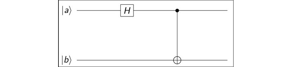
Figure 3.1 – Quantum circuit for creating a Bell state

In the preceding circuit, the Hadamard gate acts on the first qubit (|a>), and the CNOT gate acts on the output of H|a> and the second input qubit (|b>). As an exercise, show that the preceding circuit actually generates the Bell states when the first qubit |a> = {|0>, |1>} and the second qubit |b> = {|0>, |1>}.

In this section, we have demonstrated how Bell states are generated using the CNOT gate. In the next two sections, we will cover the entanglement of more than two quantum states. The next section will focus on the generation of the GHZ state. This will then be followed by a discussion of the generation of the W state.

Understanding the entanglement of more than two quantum states

In the previous section, we demonstrated how Bell states are generated using the CNOT gate. In this section, we will cover the entanglement of more than two quantum states. The next subsection will focus on the generation of the GHZ state. This will then be followed by a discussion of the generation of the W state.

Greenberger-Horne-Zeilinger state (GHZ state)

So far, we have focused on the entanglement of just two quantum states. However, in reality, many qubits can be entangled arbitrarily. One of the states that can be generated by entangling many qubits arbitrarily is the GHZ state. For n qubits, with all qubits initialized to |0>, the GHZ state is given as follows:

For three qubits, the GHZ state is given as follows:

The Python code snippet of a three-qubit GHZ state using qutip is shown as follows:

from qutip import *

GHZ = ghz_state(N=3)

print(GHZ)

Finally, the circuit for the generation of a three-qubit GHZ state, with all the input qubits (|a>, |b>, and |c>) initialized to |0>, is shown as follows:

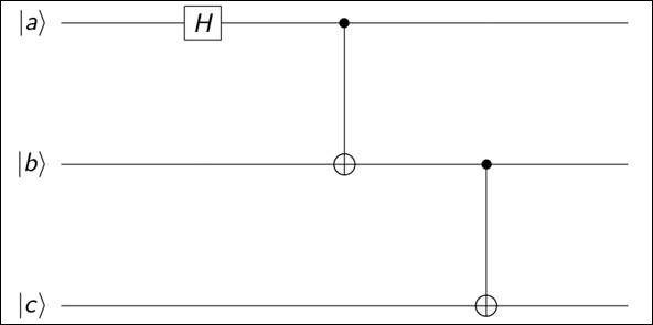
Figure 3.2 – Circuit for the generation of a three-qubit GHZ state

The W state

Besides the GHZ state, another composite quantum state that can be formed by the entanglement of three or more qubits is called the W state. A three-qubit W state is mathematically represented as follows:

In general, the W state generated from entangling n qubits is given as follows:

Finally, the Python code snippet for generating the three-qubit W state using qutip and numpy is shown here:

from qutip import *

import numpy as np

a = np.array([[1], [0]])

b = np.array([[0], [1]])

a = Qobj(a)

b = Qobj(b)

W = (1/np.sqrt(3))* (tensor(b, a, a) +

tensor(a, b, a) +

tensor(a, a, b))

print("The W state is:", W)

As can be observed, the preceding code uses two modules, namely, qutip and numpy. numpy is used to create two vectors, namely, a and b, using the array() function. These vectors are then converted into the qutip objects using the Qobj() function. Then, the W state is generated, and the W variable is assigned to such a state.

Now that we have discussed many-particle entanglement using either the GHZ states or the W states, the next section will discuss how quantum entanglement can be used as a resource in quantum information processing.

Understanding entanglement as a resource – quantum teleportation

In quantum information processing, entanglement is a crucial resource that is used to provide information processing advantages over conventional information processing. As such, quantum entanglement is typically used in various fields of quantum information processing, such as quantum cryptography, quantum computing, and quantum communication.

In quantum communication, quantum entanglement is used as a resource in applications such as superdense coding and quantum teleportation. Superdense coding will be covered in the next chapter (Chapter 4, Working with Quantum Circuits), while quantum teleportation is covered in this section. It is imperative to note that the teleportation that will be covered here is that of a quantum state, not the one that is normally talked about in sci-fi (science fiction) movies.

Quantum teleportation

Quantum teleportation involves transmitting an arbitrary quantum state from one location to another, with the assistance of an entangled EPR pair. In this quantum communication protocol, quantum entanglement is used as a key resource. As already mentioned earlier, what is teleported in this protocol is a quantum state, and not a classical object such as a human body, as is normally depicted in popular culture.

In quantum teleportation, the objective is to transfer an unknown quantum state from one point to another. This transfer is made possible through the use of an EPR pair, which is shared by Alice and Bob (remote quantum particles) and a conventional communication circuit. Therefore, the objective of quantum teleportation is to enable Alice to transmit an arbitrary quantum state to Bob. In order to achieve this, both Alice and Bob use classical communication to communicate.

The procedure for a quantum teleportation circuit can be summarized by the following circuit. This circuit uses four unitary quantum gates, namely, the Hadamard gate, the X gate, the Z gate, and the CNOT gate, together with two measurement gates:

Figure 3.3 – Circuit for quantum teleportation

As can be observed from the diagram, Alice has the unknown state |ψ> and one half of the EPR pair that she shares with Bob. She then performs a measurement on the two qubits at her disposal, and sends the results of the measurement to Bob through a classical channel. Since she is measuring two qubit states, Alice's possible measurement outcomes m1 (from the qubit to be transmitted) and m2 (from one half of the EPR pair) are 00, 01, 10, or 11.

Based on the value of the measurement outcome received from Alice, Bob can perform any of the operations shown in the following table in order to reconstruct the state |ψ>:

Figure 3.4 – Table showing operations that can be performed by Bob based on the value of measurement outcome received from Alice

Using IBM's Qiskit platform and Google's Colab environment, the following Python code can be used to implement quantum teleportation:

#!pip install qiskit

from qiskit import *

from qiskit.visualization import plot_histogram

circuit = QuantumCircuit(3,3)

circuit.h(0)

circuit.h(1)

circuit.cx(1,2)

circuit.cx(0,1)

circuit.h(0)

circuit.measure([0, 1], [0, 1])

circuit.cx(1, 2)

circuit.cz(0, 2)

circuit.measure([2], [2])

circuit.draw(output='text')

simulator = Aer.get_backend('qasm_simulator')

result = execute(circuit, backend=simulator,

shots=1024).result()

plot_histogram(result.get_counts(circuit))

The code can be summarized as follows. The code uses the qiskit Python module. After importing the qiskit module into the workspace, the circuit is instantiated using the QuantumCircuit() function, and the circuit variable is assigned to this instantiated circuit. This circuit uses three quantum registers and three classical registers. After instantiating the circuit, the unitary circuits are then applied to the quantum states. Finally, a measurement is performed and the results stored in the classical registers. The final part of the code, starting from the circuit.draw(output='text') statement to the end, is just used for the visualization of the quantum teleportation circuit generated.

Summary

In this chapter, we have covered the basics of quantum entanglement. We have also seen the inequalities that can be used to determine the quantumness of the correlations. These inequalities are the Bell inequality and the CHSH inequality.

Additionally, we introduced the Bell basis states. Furthermore, we learned in this chapter that the CNOT gate is the quantum gate that is responsible for entanglement, hence it can also be referred to as the entangling gate.

In this chapter, we also covered the entangled states of more than two entangled qubits, and these states are the GHZ and W states. Additionally, we argued in this chapter that quantum entanglement is a crucial resource for quantum information processing applications. Finally, we provided a hands-on introduction to quantum teleportation.

The next chapter provides a hands-on exposition to various quantum circuits. It also discusses an implementation of a superdense coding quantum communication protocol.

Further reading

• Wilde, M. M. (2017). Quantum Information Theory. Cambridge University Press.
• Bell, J. S. (1987). Speakable and Unspeakable in Quantum Mechanics. Cambridge University.
• Bertlmann, R., and Zeilinger, A. (2017). Quantum [Un] Speakables II. Berlin: Springer.