
SQL Server default configuration allows you to run noncritical applications with little knowledge or administrative effort. This is especially true for applications running the lower Stock Keeping Units (SKUs) of the product such as SQL Server Express edition. However, for most production applications, you need to follow a database implementation cycle consisting of four steps: design, configuring, monitoring, and troubleshooting. This is extremely important for mission-critical applications where areas such as performance, availability, or security are an essential requirement. I want to emphasize that this is a cycle as well. Once these four steps are successfully completed and the application goes live, it does not end there. Monitoring is vitally important. As the workload, database, or application changes—or even during regular activity—problems will arise that may require a new thinking, design, and configuration, going back to the aforementioned cycle again. This book focuses on performance and will guide you through all the four areas, giving you the tools and knowledge required to get the best performance out of your databases.
Before getting into the four areas, this introductory chapter explains how the SQL Server database engine works and covers everything that happens in the system from the moment a client makes a connection using the Tabular Data Stream (TDS) protocol over a network protocol until a query is executed and the results are returned to the client. Although so many things could happen in the middle and may require an entire book to cover it, I focus on the work performed by SQLOS, the relational engine, which consists of the query optimizer and the execution engine, and other important performance-related factors like memory grants, lock, and latches. The content of this chapter is the foundation for the rest of the book.
This book does not explicitly cover query tuning and optimization, so you don’t have to be an advanced query writer or understand execution plans to use it. This book can help database administrators, architects, and database developers to better understand how SQL Server works and what to do to fix performance problems. For information on query tuning and optimization, you can refer to my book Microsoft SQL Server 2014 Query Tuning & Optimization (McGraw-Hill Education, 2015).
TDS/Network Protocols
SQL Server is a client-server platform in which a client usually establishes a long-lived connection with the database server using the Tabular Data Stream (TDS) protocol over a network protocol. TDS is an application-level protocol that facilitates the interaction between clients and SQL Server. Sybase Inc. initially designed and developed it for their Sybase SQL Server relational database engine in 1984, which later became a Microsoft product. Although the TDS specification does not define a specific network transport protocol, the current version of TDS has been implemented over the TCP/IP and Named Pipes network transport protocols. The Virtual Interface Architecture (VIA) network protocol was deprecated but still available on older versions of SQL Server. It was finally removed with SQL Server 2016.
You can also use the Shared Memory protocol to connect to an instance of SQL Server, but it can only be used to connect from the same computer where the database engine is running; it cannot be used for access from other computers on the network.
TDS provides several functions including authentication and identification, channel encryption negotiation, specification of requests in SQL and bulk insert operations, invocation of a stored procedure or user-defined function, and the return of data. Open Database Connectivity (ODBC), Java Database Connectivity (JDBC), and Object Linking and Embedding Database (OLE DB) are libraries that use TDS to transfer data between the client and SQL Server. TDS requests and responses between a client and SQL Server can be inspected by using different network protocol analyzer tools such as Wireshark. Another popular tool, Microsoft Message Analyzer (MMA), was retired as of November of 2019.
SQL Batch: To send a SQL statement or a batch of SQL statements
Remote procedure call: To send a remote procedure call containing the stored procedure or user-defined function name, options, and parameters
Bulk load: To send a SQL statement for a bulk insert/bulk load operation
Note that a stored procedure or user-defined function name can be requested through either a remote procedure call or a SQL batch. For more details about TDS, you can find the TDS specification at https://msdn.microsoft.com/en-us/library/dd304523.aspx.
TCP/IP is by far the most common protocol used by SQL Server implementations. The default TCP/IP port used by the database engine is 1433, although other ports can be configured and are in some cases required, for example, when running multiple instances on the same server. Some other services may use a different port. For example, the SQL Server Browser starts and claims UDP port 1434. When the SQL Server database engine uses a TCP/IP port different from the default, the port number has to either be specified in the connection string at the client or it can be resolved by the SQL Server Browser service, if enabled. The default pipe, sqlquery, is used when Named Pipes protocol is configured.
ODBC: ODBC (Open Database Connectivity) is an open standard API based on the Call-Level Interface (CLI) specifications originally developed by Microsoft during the early 1990s. ODBC has become the de facto standard for data access in both relational and nonrelational database management systems.
OLE DB: OLE DB (Object Linking and Embedding Database) is an API designed by Microsoft for accessing not only SQL-based databases but also some other different data sources in a uniform matter. Even though OLE DB was originally intended as a higher-level replacement for and successor to ODBC, ODBC remains the most widely used standard for database access.
JDBC: JDBC (Java Database Connectivity) is an API developed by Sun Microsystems that defines how a client can access a relational database from the Java programming language. JDBC is part of the Java standard edition platform, which has since been acquired by Oracle Corporation.
ADO.NET: ADO.NET (ActiveX Data Objects for .NET) is a set of classes that expose data access services and is an integral part of the Microsoft .NET framework. ADO.NET is commonly used to access data stored in relational database systems though it can access nonrelational sources as well.
How Work Is Performed
Now that we have seen how a client connects to the database server, we can review what happens next and see how the work requested by the client is performed. In SQL Server, each user request is an operating system thread, and when a client connects, it is assigned to a specific scheduler. Schedulers are handled at the SQLOS level, which also handles tasks and workers, among other functions. Moving a level higher, we have connections, sessions, and requests. Let’s review schedulers, tasks, and workers by first introducing SQLOS.
SQLOS
SQLOS is the SQL Server application layer responsible for managing all operating system resources which includes managing nonpreemptive scheduling, memory and buffer management, I/O functions, resource governance, exception handling, and extended events. SQLOS performs these functions by making calls to the operating system on behalf of other database engine layers or, like in the cases of scheduling, by providing services optimized for the specific needs of SQL Server.
SQL Server schedulers were introduced with SQL Server 7 since before that version it relied on the Windows scheduling facilities. The main question here is why there is the need for SQLOS or a database engine to replace available operating system services. Operating system services are general-purpose services and sometimes inappropriate for database engine needs as they do not scale well. Instead of using generic scheduling facilities for any process, scheduling can be optimized and tailored to the specific needs of SQL Server. The main difference between the two is that a Windows scheduler is a preemptive scheduler, while SQL Server is a cooperative scheduler or nonpreemptive one. This improves scalability as having threads voluntarily yield is more efficient than involving the Windows kernel to prevent a single thread from monopolizing a processor.
In Operating System Support for Database Management, Michael Stonebraker examines whether several operating system services are appropriate for support of database management functions like scheduling, process management, and interprocess communication, buffer pool management, consistency control, and file system services. You can find this publication online at www.csd.uoc.gr/~hy460/pdf/stonebreaker222.pdf.
Schedulers
Schedulers schedule tasks and are mapped to an individual logical processor in the system. They manage thread scheduling by allowing threads to be exposed to individual processors, accepting new tasks, and handing them off to workers to execute them (workers are described in more detail shortly). Only one worker at a time can be exposed to an individual logical processor, and, because of this, only one task on such processor can execute at any given time.
Schedulers that execute user requests have an ID number less than 1048576, and you can use the sys.dm_os_schedulers DMV (Dynamic Management View) to display runtime information about them. When SQL Server starts, it will have as many schedulers as the number of available logical processors to the instance. For example, if in your system SQL Server has 16 logical processors assigned, sys.dm_os_schedulers can show scheduler_id values going from 0 to 15. Schedulers with IDs greater than or equal to 1048576 are used internally by SQL Server, such as the dedicated administrator connection scheduler, which is always 1048576. (It was 255 on versions of SQL Server 2008 and older.) These are normally referred to as hidden schedulers and, as suggested, are used for processing internal work. Schedulers do not run on a particular processor unless the processor affinity mask is configured to do so.

Task execution process
As mentioned earlier, in SQL Server, a scheduler runs in a nonpreemptive mode, meaning that a task voluntarily releases control periodically and will run as long as its quantum allows it or until it gets suspended on a synchronization object (a quantum or time slice is the period of time for which a process is allowed to run). Under this model, threads must voluntarily yield to another thread at common points instead of being randomly context-switched out by the Windows operating system. The SQL Server code was written so that it yields as often as necessary and in the appropriate places to provide better system scalability.
Figure 1-1 shows that a task can also run in preemptive mode, but this will only happen when the task is running code outside the SQL Server domain, for example, when executing an extended stored procedure, a distributed query, or some other external code. In this case, since the code is not under SQL Server control, the worker is switched to preemptive mode, and the task will run in this mode as it is not controlled by the scheduler. You can identify if a worker is running in preemptive mode by looking at the is_preemptive column of the sys.dm_os_workers DMV.
The lightweight pooling option is an advanced configuration option. If you are using the sp_configure system stored procedure to update the setting, you can change lightweight pooling only when show advanced options is set to 1. The setting takes effect after the server is restarted. Of course, if you try this in your test environment, don’t forget to set it back to 0 before continuing. Looking at the is_fiber column on the sys.dm_os_workers DMV will show if the worker is running using lightweight pooling.
Workers
PENDING: Waiting for a worker thread
RUNNABLE: Runnable, but waiting to receive a quantum
RUNNING: Currently running on the scheduler
SUSPENDED: Has a worker, but is waiting for an event
DONE: Completed
SPINLOOP: Stuck in a spinlock
Similarly, you can find additional information about tasks waiting on some resource by using sys.dm_os_waiting_tasks. We will cover waits in great detail in Chapter 5.
Max Worker Threads Default Configuration
Number of CPUs | 32-Bit Architecture (Up to SQL Server 2014) | 64-Bit Architecture (Up to SQL Server 2016 SP1) | 64-Bit Architecture (Starting with SQL Server 2016 SP2) |
|---|---|---|---|
4 or fewer processors | 256 | 512 | 512 |
8 processors | 288 | 576 | 576 |
16 processors | 352 | 704 | 704 |
32 processors | 480 | 960 | 960 |
64 processors | 736 | 1472 | 2432 |
128 processors | 1248 | 2496 | 4480 |
256 processors | 2272 | 4544 | 8576 |
Starting with SQL Server 2016, the database engine is no longer available on a 32-bit architecture.
Workers are created in an on-demand fashion until the “max worker threads” configured value is reached (according to the value shown in Table 1-1 for a default configuration), although this value does not take into account threads that are required for system tasks. As shown earlier, the max_workers_count column on the sys.dm_os_sys_info DMV will show the maximum number of workers that can be created.
The scheduler will trim the worker pool to a minimum size when workers have remained idle for more than 15 minutes or when there is memory pressure. For load-balancing purposes, the scheduler has an associated load factor that indicates its perceived load and that is used to determine the best scheduler to put this task on. When a task is assigned to a scheduler, the load factor is increased. When a task is completed, the load factor is decreased. This value can be seen on the load_factor column of the sys.dm_os_schedulers DMV.
A ring buffer is a circular data structure of a fixed size.
Having reviewed schedulers, tasks, and workers, let’s move to a level higher and discuss connections, sessions, and requests.
You can use the sys.dm_exec_connections DMV to see the physical connections to the database server. Some of the interesting information is found in the net_transport column, which shows the physical transport protocol used by this connection such as TCP, Shared Memory, or Session (when a connection has multiple active result sets, or MARS, enabled); protocol_type, which is self-explanatory and could have values like TSQL; Service Broker or SOAP; and some other important information like network address of the client connecting to the database server and the port number on the client computer for TCP/IP connections. There is a one-to-one mapping between a connection and a session, as shown in Figure 1-2.
Schedulers, workers, and tasks are objects at the SQLOS level and as such are included in the SQL Server operating system–related DMVs, as compared to connections, sessions, and requests, which are included in the execution-related DMV group.
Running: Currently running one or more requests.
Sleeping: Currently connected but running no requests.
Dormant: The session has been reset because of connection pooling and is now in pre-login state.
Preconnect: The session is in the Resource Governor classifier.
Finally, sys.dm_exec_requests is a logical representation of a query request made by the client at the execution engine level. It provides a great deal of rich information including status of the request (which can be Background, Running, Runnable, Sleeping, or Suspended), hash map of the SQL text and execution plan (sql_handle and plan_handle, respectively), wait information, and memory allocated to the execution of a query on the request. It also provides a lot of rich performance information like CPU time in milliseconds, total time elapsed in milliseconds since the request arrived, number of reads, number of writes, number of logical reads, and number of rows that have been returned to the client by this request.
The sys.dm_exec_session_wait_stats DMV, available since SQL Server 2016, can allow you to collect wait information at the session level. More details of this DMV will be provided in Chapter 5.

Execution-related DMV mapping
SQL Server on Linux
As you may probably know, starting with the 2017 version, SQL Server now runs on Linux, more specifically on Red Hat Enterprise Linux, SUSE Linux Enterprise Server, and Ubuntu. In addition, SQL Server can run on Docker. Docker itself runs on multiple platforms, which means it is possible to run a SQL Server Docker image on Linux, Mac, or Windows.
Although SQLOS was created to remove or abstract away operating system differences, it was never originally intended to provide platform independence or portability or to help porting the database engine to other platforms. But even when SQLOS did not provide the abstraction functionality to move SQL Server to another operating system, it would still play a very important role on the Linux release.
SQL Server on Linux is not a native Linux application but instead uses the Drawbridge application sandboxing technology. This means Drawbridge provided the abstraction functionality that was needed. SQL Server on Linux was born from marrying these two technologies, SQLOS and Drawbridge, and was the birth of a new platform abstraction layer later known as SQLPAL. How SQL Server on Linux works is explained in more detail in Chapter 2.
Query Optimization
We have seen how schedulers and workers execute tasks once a request has been submitted to SQL Server. After an idle worker picks up a pending task, the submitted query has to be compiled and optimized before it can be executed. To understand how a query is executed, we now switch from the world of SQLOS to the work performed by the relational engine, which is also called the query processor and consists of two main components: the query optimizer and the execution engine. The job of the query optimizer is to assemble an efficient execution plan for the query using the algorithms provided by the database engine. After a plan is created, it will be executed by the execution engine.
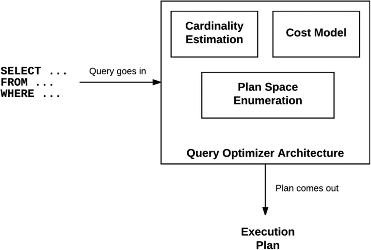
Query optimizer architecture

SQL Server query processing process
The query processing process follows several steps, as shown in Figure 1-4, although the main optimization process is performed by up to three exploration stages at the end. This is the part where transformation rules are used to produce candidate plans and cardinalities and costs are estimated. The optimization process does not have to execute all three exploration phases and could stop at any of them as soon as a good execution plan is found.
In addition to the query text, which at this moment has been translated into a tree of logical operations and the metadata related to the objects directly related to the query, the query optimizer will collect additional information from other objects like constraints, indexes, and so on, along with optimizer statistics.
Join Orders for Left-Deep and Bushy Trees
Tables | Left-Deep Trees | Bushy Trees |
|---|---|---|
2 | 2 | 2 |
3 | 6 | 12 |
4 | 24 | 120 |
5 | 120 | 1,680 |
6 | 720 | 30,240 |
7 | 5,040 | 665,280 |
8 | 40,320 | 17,297,280 |
9 | 362,880 | 518,918,400 |
10 | 3,628,800 | 17,643,225,600 |
11 | 39,916,800 | 670,442,572,800 |
12 | 479,001,600 | 28,158,588,057,600 |
Names like left-deep, right-deep, and bushy trees are commonly used to identify the shapes of the order of joins in logical trees. Left-deep trees are also called linear trees or linear processing trees. The set of bushy trees includes the sets of both left-deep and right-deep trees. For more details, you can look at my post at www.benjaminnevarez.com/2010/06/optimizing-join-orders/.
In order to explore the search space, a plan enumeration algorithm is required to explore semantically equivalent plans. The generation of equivalent candidate solutions is performed by the query optimizer by using transformation rules. Heuristics are also used by the query optimizer to limit the number of choices considered in order to keep the optimization time reasonable. The set of alternative plans considered by the query optimizer is referred to as the search space and is stored in memory during the optimization process in a component called the memo.
After enumerating candidate plans, the query optimizer needs to estimate the cost of these plans so it can choose the optimal one, the one with the lowest cost. The query optimizer estimates the cost of each physical operator in the memo structure, using costing formulas considering the use of resources such as I/O, CPU, and memory, although only the CPU and I/O costs are reported in the operators as can be seen later on the query plan. The cost of all the operators in the plan will be the cost of the query. The cost estimation is by operator and will depend on the algorithm used by the physical operator and the estimated number of records that will need to be processed. This estimate of the number of records is known as the cardinality estimation.
Cardinality estimation uses a mathematical model that relies on statistical information and calculations based on simplifying assumptions like uniformity, independence, containment, and inclusion (which still holds true for the new cardinality estimator introduced with SQL Server 2014). Statistics contain information describing the distribution of values in one or more columns of a table that consists of histograms, a global calculated density information, and optionally special string statistics (also called tries). Cardinality for the base table can be obtained directly using statistics, but estimation of most other cardinalities—for example, for filters or intermediate results for joins—has to be calculated using predefined models and formulas. However, the model does not account for all the possible cases, and sometimes, as mentioned earlier, assumptions are used. Statistics are, by default, created and updated automatically by SQL Server, and administrators have multiple choices to manage them as well.
Most of the internal information about what the SQL Server query optimizer does can be inspected using undocumented statements and trace flags, although these are not supported by Microsoft and are not intended to be used in a production system. We will cover some of them in the rest of the chapter.
Since our interest in this chapter is to understand how SQL Server works, after this introduction, let us now review the query optimization process in more detail, starting with parsing and binding.
Parsing and Binding
As mentioned earlier, parsing and binding are the first operations performed when a query is submitted for execution. Parsing checks the query for correct syntax, including the correct use of keywords and spelling, and translates its information into a relational algebra tree representing the logical operators of the query.
Most of the examples in this book use the AdventureWorks databases, which you can download from https://docs.microsoft.com/en-us/sql/samples/adventureworks-install-configure. Download both AdventureWorks2017.bak and AdventureWorksDW2017.bak backup files, which are the OLTP (Online Transaction Processing) and data warehouse databases, and restore them in SQL Server as AdventureWorks2017 and AdventureWorksDW2017. All the code in this book has been tested in SQL Server 2019 so you also want to make sure to change these databases’ compatibility level to 150.
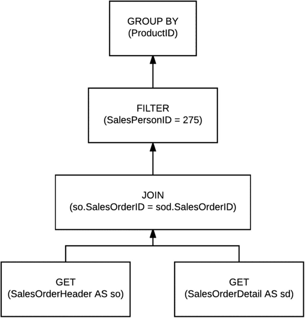
Query tree representation
Name resolution for views also includes the process of view substitution in which a view reference is expanded to include the actual view definition. The query tree representation, as shown in Figure 1-5, represents the logical operations performed by the query and is closely related to the original syntax of the query. These logical operations include things like “get data from the Sales table,” “perform an inner join,” “perform an aggregation,” and so on. The query processor will use different tree representations during the entire optimization process, and these trees will have different names.
The following is the output of such query on SQL Server 2019 Cumulative Update 4. The @@VERSION function in my system in addition returns Microsoft SQL Server 2019 (RTM-CU4) (KB4548597) - 15.0.4033.1 (X64) where KB4548597 is the knowledge base article describing the cumulative update and 15.0.4033.1 is the product version. Starting with SQL Server 2017, service packs are no longer available, and the new servicing model will be based on cumulative updates (and General Distribution Releases, or GDRs, when required), and only CU are released.
Note: Cumulative updates are intended to be released more frequently after the original release (called RTM or Release to Manufacturing) and then less often in this new service model. A cumulative update will be available every month for the first 12 months and then every 2 months for the remaining 4 years of the full 5-year mainstream life cycle. For more details about this new servicing model, you can look at https://techcommunity.microsoft.com/t5/sql-server/announcing-the-modern-servicing-model-for-sql-server/ba-p/385594 (or search for “Announcing the Modern Servicing Model for SQL Server”).
map_key | map_value |
|---|---|
0 | CONVERTED_TREE |
1 | INPUT_TREE |
2 | SIMPLIFIED_TREE |
3 | JOIN_COLLAPSED_TREE |
4 | TREE_BEFORE_PROJECT_NORM |
5 | TREE_AFTER_PROJECT_NORM |
6 | OUTPUT_TREE |
7 | TREE_COPIED_OUT |
In this case, QUERYTRACEON is a query hint that lets you enable a plan-affecting trace flag at the query level. As we know, a trace flag is a well-known mechanism used to set specific server characteristics or to alter a particular behavior in SQL Server.
Note: The QUERYTRACEON query hint was undocumented and unsupported for many years and only recently has been supported but only with a limited number of the available trace flags. You can get more information about the trace flags supported by QUERYTRACEON by looking at the documentation at https://docs.microsoft.com/en-us/sql/t-sql/queries/hints-transact-sql-query.
Finally, a reminder that this book, especially this chapter, includes many undocumented and unsupported features and statements. As such, you can use them in a test environment for learning or troubleshooting purposes, but they are not meant to be used in a production environment. Using them in your production environment could make it unsupported by Microsoft. I will identify when a statement, feature, or trace flag is undocumented and unsupported.
Although the listed relational algebra operations are not documented in any way and may be even hard to read in such a cryptic text format, we could identify that the three main operations of the query, which are the SELECT, FROM, and WHERE clauses, correspond to the relational algebra operations Project or LogOp_Project, Get or LogOp_Get, and Select or LogOp_Select, respectively. To make things even more complicated, the LogOp_Select operation is not related to the SELECT clause but has to do more with the filter operation or WHERE clause. LogOp_Project is used to specify the columns required in the result. Finally, LogOp_Get specifies the table used in the query.
In summary, trace flag 8605 can be used to display the query initial tree representation created by SQL Server, trace flag 8606 will display additional logical trees used during the optimization process (e.g., the input tree, simplified tree, join-collapsed tree, tree before project normalization, or tree after project normalization), and trace flag 8607 will show the optimization output tree. For more details about these trace flags, you can look at the following post at my blog at www.benjaminnevarez.com/2012/04/more-undocumented-query-optimizer-trace-flags.
After parsing and binding are completed, the real query optimization process starts. The query optimizer will obtain the generated logical tree and will start with the simplification process.
Simplification
- A)
Predicate pushdown: In this simplification optimization, filters in WHERE clauses may be pushed down in the logical query tree in order to enable early data filtering. This process can also help on better matching of indexes and computed columns later in the full optimization process.
- B)
Contradiction detection: Contradictions are detected and removed on this step. Contradictions can be related to check constraints or how the query is written. By removing redundant operations on a query, query execution is improved, as there is no need to spend resources on unnecessary operations. For example, removing access to a non-needed table can save I/O resources.
- C)
Simplification of subqueries: Subqueries are converted into joins. However, since subqueries do not always translate directly to an inner join, group by and outer join operations may be added as necessary.
- D)
Redundant joins removal: Redundant inner and outer joins could be removed. Foreign key join elimination is an example of this simplification. When foreign key constraints are available and only columns of the referencing table are requested, a join can potentially be removed.

Plan for a VacationHours predicate

Contradiction detection
This very simple plan with a single constant scan operation basically means that the query optimizer decided not to create a plan at all. Because of the check constraint, the query optimizer knows there is no way the query can return any records at all and create a constant scan operator which is not really performing any work at all.
After disabling the check constraint, if you run the last query again (using the VacationHours > 300 predicate), you should see again the execution plan shown in Figure 1-6 where a clustered index scan is needed. Without the check constraint, SQL Server has no other choice but to scan the table and perform the filter to validate if any records with the requested predicate exist at all.
Once again, this query represents an obvious contradiction, since those two predicate conditions could never exist at the same time. The query will return no data, but more importantly it would not take any time at all for the query processor to figure it out, and the plan created will be just another constant scan as shown in Figure 1-7. You may still argue that nobody would ever write such a query, but this is a very simple example just to show the concept. The query optimizer would still find the problem in very complicated queries with multiple tables and predicates or even if one predicate is in one query and the contradicting predicate is on a view.
After the simplification part is completed, we could finally move to the full optimization process. But first, what about a check to validate if an optimization is required after all?
Trivial Plan Optimization
There may be cases in which a full optimization is not required. This could be the case for very simple queries in which the plan choice may be very simple or obvious. The query optimizer has an optimization called trivial plan which can be used to avoid the expensive optimization process. As mentioned earlier, the optimization process may be expensive to initialize and run.
When you run such query, you can request an execution plan to confirm it is a trivial plan.
Note: There are several ways to request an estimated or actual execution plan. To request an actual graphical execution plan, select “Include Actual Execution Plan” (or Ctrl-M) on the SQL Server Management Studio toolbar. Once you have a graphical execution plan, you can right-click it and select “Show Execution Plan XML …”. For more details about execution plans, see the documentation at https://docs.microsoft.com/en-us/sql/relational-databases/performance/execution-plans.
If a plan does not qualify for a trivial optimization, StatementOptmLevel would show the value FULL which means that a full optimization was instead required.
Finally, if the query did not qualify for a trivial plan, the query optimizer will perform a full optimization. We will cover that next in this section. But first, as mentioned earlier, a query could potentially have millions of possible candidate execution plans. So, we need choices to create alternate plans and to purge plans most likely not needed. Transformation rules create alternate plans. Some defined heuristics purge or limit the number of plans considered. Transformation rules are the fundamental algorithm for these kinds of optimizers. In fact, some optimizers are even called rule-based optimizers. However, even when the SQL Server optimizer uses rules to search for alternate plans, it is actually called a cost-based optimizer, as the final decision about selecting a plan will be a cost-based decision. So, let us talk about transformation rules next .
Transformation Rules
As mentioned previously, the SQL Server query optimizer uses transformation rules to produce alternate execution plans. A final execution plan would be later chosen after cardinalities and costs are estimated. Transformation rules are based on relational algebra operations. The query optimizer will apply transformation rules to the previously generated logical tree of operators and by doing that would create additional equivalent logical and physical alternatives. In other words, it will take a relational operator tree and would generate equivalent relational trees.
At the beginning of the optimization process, as we saw earlier, a query tree contains only logical expressions. Once transformation rules are applied, they could generate additional logical and physical expressions. A logical expression could be, for example, the definition of a join, as in the SQL language, and the physical expression would be when the query optimizer selects one of the physical operators like nested loops join, merge join, or hash join. In a similar way, a logical aggregate operation could be implemented with two physical algorithms, stream aggregate and hash aggregate.
Transformation rules could be categorized in three types, simplification, exploration, and implementation rules. Simplification rules are mostly used in the simplification phase, which we covered earlier, and their purpose is to simplify the current logical tree of operations. Exploration rules, which are also called logical transformation rules, are used to generate equivalent logical alternatives. On the other side, implementation rules, which are also called physical transformation rules, are used to generate equivalent physical alternatives.
All the logical and physical alternatives generated during the query optimization process are stored in a memory structure called the memo. But keep in mind that finding alternatives is just solving one part of the problem. There is still the need to select the best choice. A cost estimation component will estimate the cost of the physical operations (there is no need to estimate the cost of logical operations). Even when all the alternate plans are equivalent and would produce the same query results, their costs could be dramatically different. Obviously, a bigger cost means using more resources such as CPU, I/O, or memory, impacting the query performance, hence the responsibility to select the best or lower cost.
Finally, keep in mind that the query optimization process is extremely complicated, and by that it is not perfect. For example, it could be possible that an optimal plan may not be generated at all as a specific query could produce millions and millions of plans, and many of those may be discarded or not considered at all. Or perhaps it could be possible that the perfect plan may be generated and stored in the memo structure but not selected at all because of an incorrect cost estimation which instead selects another plan.
name | promise_total |
|---|---|
JNtoNL | 721299 |
LOJNtoNL | 841440 |
LSJNtoNL | 32803 |
LASJNtoNL | 26609 |
JNtoSM | 1254182 |
FOJNtoSM | 5448 |
LOJNtoSM | 318398 |
ROJNtoSM | 316128 |
LSJNtoSM | 9414 |
RSJNtoSM | 9414 |
LASJNtoSM | 10896 |
RASJNtoSM | 10896 |
There is not much about transformation rules or how they work in the SQL Server documentation. But there are also some undocumented statements which could allow you to inspect and learn more about transformation rules and the optimization process in general.

Group by aggregate before join optimization
As shown in Figure 1-8, assuming we originally have the logical tree on the left, after applying the GbAggBeforeJoin rule, the query optimizer is able to generate the logical tree on the right. The traditional query optimization for this kind of query would be to perform the join on both tables first and then perform the aggregation using the join results. In some cases, however, performing the aggregation before the join could be more efficient.
Both trees in Figure 1-8 are equivalent and, if executed, would produce exactly the same results. But, as mentioned more than once so far, one tree or execution plan could be more efficient than the other, and that is the reason we are optimizing this (and the reason query optimizers exist in the first place).

Plan with group by aggregate before join optimization
We have another undocumented way to play with these rules which can help us better understand how they work. But be careful, these are undocumented statements and, as such, should never be used in a production environment. I would not even recommend using them in any other shared environment even if it is nonproduction. But feel free to use them in your personal installation of SQL Server for learning or troubleshooting purposes.

Plan with GbAggBeforeJoin rule disabled
In this plan, we can see that the GbAggBeforeJoin optimization has been disabled, and the best plan found shows that the aggregation is now after the join. If you wonder why one plan was chosen against the other, you may want to check at the cost of the plan. The cost of the original plan is 0.309581, while the cost of the plan without the GbAggBeforeJoin optimization is 0.336582, so clearly the original is the winner. In cost, lower values are better, obviously. Although the numbers may not show a big difference, keep in mind these are very small tables and the difference would be bigger on real production databases.

Plan without the Join to Sort Merge Join optimization

Plan without hash aggregations
After enabling the listed transformation rules, you can run the query again and verify that everything goes back to normal. You can also run DBCC SHOWOFFRULES to verify that no rules are listed as disabled at all.
Using hints may have the same or very similar behavior, but this time it is allowed and documented; however, it is not recommended unless you have really good reasons to do so. By the way, the FORCE ORDER hint specifies that the join order and aggregation placement indicated by the query syntax is preserved during query optimization.
The Memo
As indicated earlier, the memo is a memory structure used to store the alternatives generated and analyzed by the query optimizer. A new memo structure is created for each optimization, and it is only kept during the optimization process. Initially, the original logical tree created during parsing and binding will be stored in the memo. As transformation rules are applied during the optimization process, the new logical and physical operations will be stored here.
As expected, the memo will store all the logical and physical operations created while applying transformation rules, as discussed before. The cost estimation component will estimate the cost of the physical operations stored here. There is no need to estimate the cost of logical operations.
You can also try at your own risk the same query with undocumented trace flag 8615 to display the final memo structure.
Full Optimization
We just reviewed how transformation rules work. Now let us define how the full optimization process works. As defined earlier, query optimization uses transformation rules to produce alternate equivalent plans and operations and heuristics to purge or limit the number of plans considered. A cost estimation component is also required to select the best plan. Remember, in our previous example, just a simple optimization such as moving a group by aggregate before the join changed the cost of the plan from 0.336582 to 0.309581 (more on cost estimation and the meaning of this cost value later).
We also saw that the sys.dm_exec_query_transformation_stats DMV lists all the possible transformation rules which can be used by the query optimizer. Obviously, the query optimizer does not run all the transformation for every single query; it runs the transformations required depending on the query features. It will apply transformation related to joins to queries performing joins, transformation rules about aggregations only if the query uses aggregations, and so on. There will never be a need to apply rules for star join queries, columnstore indexes, or windowing functions to our previous example as they are not used by the query at all.
Search 0 or transaction processing phase: This phase will try to find a plan as quickly as possible without trying sophisticated transformations. This phase is optimal for small queries typically found on transaction processing systems, and it is used for queries with at least three tables.
Search 1 or quick plan: Search 1 uses additional transformation rules, limited join reordering, and it is more appropriate for complex queries.
Search 2 or full optimization: Search 2 is used for queries ranging from complex to very complex. A larger set of potential transformation rules, parallel operators, and other advanced optimization strategies are considered in this phase.
There are a few ways, some documented and some undocumented, to see which phases are executed during a specific query optimization. Let us start with the documented way, or rather partially documented, which is using the sys.dm_exec_query_optimizer_info DMV.
The sys.dm_exec_query_optimizer_info DMV is very interesting in many other ways, so I will discuss a few of them later in this section too.
counter | occurrence | value |
|---|---|---|
optimizations | 105870900 | 1 |
elapsed time | 105866079 | 0.006560191 |
final cost | 105866079 | 74.81881849 |
trivial plan | 39557103 | 1 |
tasks | 66308976 | 1277.59664 |
no plan | 0 | NULL |
search 0 | 13235719 | 1 |
search 0 time | 17859731 | 0.006893007 |
search 0 tasks | 17859731 | 1188.208326 |
search 1 | 52398882 | 1 |
search 1 time | 55005619 | 0.002452487 |
search 1 tasks | 55005619 | 578.9377145 |
search 2 | 674375 | 1 |
search 2 time | 1577353 | 0.09600762 |
search 2 tasks | 1577353 | 20065.39848 |
gain stage 0 to stage 1 | 4621326 | 0.252522572 |
gain stage 1 to stage 2 | 673774 | 0.032957197 |
timeout | 3071016 | 1 |
memory limit exceeded | 0 | NULL |
insert stmt | 36405807 | 1 |
delete stmt | 3331067 | 1 |
update stmt | 7395325 | 1 |
merge stmt | 72030 | 1 |
contains subquery | 3791101 | 1 |
unnest failed | 9177321 | 1 |
tables | 105870900 | 2.094998408 |
hints | 1528603 | 1 |
order hint | 1493599 | 1 |
join hint | 717606 | 1 |
view reference | 10142222 | 1 |
remote query | 779911 | 1 |
maximum DOP | 105870900 | 7.888350765 |
maximum recursion level | 229 | 0 |
indexed views loaded | 63 | 1 |
indexed views matched | 147 | 1 |
indexed views used | 0 | NULL |
indexed views updated | 0 | NULL |
dynamic cursor request | 4151 | 1 |
fast forward cursor request | 361 | 1 |
Don’t be intimidated by the long output; there is a lot of rich information here. This DMV provides insight about the optimizations and work performed by the query optimizer on the current instance. It is worth noticing that the DMV provides cumulative statistics collected since the SQL Server instance was started. Sadly, this DMV used to be fully documented (up to SQL Server 2005), but later versions of the documentation omit descriptions of nearly half of the listed counters and only label them as “Internal only.” For example, the entry “trivial plan” used to have the description “Total number of trivial plans (used as final plan)” where now it shows “Internal only.” You can find this DMV documentation at https://docs.microsoft.com/en-us/sql/relational-databases/system-dynamic-management-views/sys-dm-exec-query-optimizer-info-transact-sql.
As an example, the previous output shows that there have been 105,870,900 optimizations since the SQL Server instance started, that the average elapsed time for each optimization was 0.006560191 seconds, and that the average estimated cost of each optimization, in internal cost units, was about 74.81881849. Most of the optimizations in this system went through search 0 and 1 phases.
A lot of other useful information about optimizations could be found here, for example, it would be important to know the number of optimizations on your system involving hints, order hints, join hints, trivial plans, timeouts, subqueries, maximum DOP, and so on.
counter | occurrence | value |
|---|---|---|
elapsed time | 2 | 0 |
final cost | 2 | 0.708588242 |
insert stmt | 1 | 1 |
maximum DOP | 2 | 16 |
optimizations | 2 | 2 |
search 0 | 1 | 1 |
search 0 tasks | 1 | 383 |
search 0 time | 1 | 0.001 |
search 1 | 1 | 1 |
search 1 tasks | 2 | 341 |
search 1 time | 2 | 0 |
tables | 2 | 5 |
tasks | 2 | 724 |
timeout | 1 | 1 |
view reference | 1 | 1 |
All three methods show that this particular query went through two phases of the query optimization process, transaction processing and quick plan.
Cost Estimation
As mentioned earlier , the quality of the execution plans the query optimizer generates is directly related to the quality of the equivalent plans produced and the accuracy of their cost estimates. This means that even when the query optimizer is able to produce a perfect execution plan for a query (and have it stored in the memo), an incorrect cost estimation may lead to the query optimizer choosing another less efficient plan.
The query optimizer uses costing formulas considering the use of resources such as I/O, CPU, and memory, and the resulting values may look like a mystery for many. For example, you may be surprised that cost estimation does not consider if your query has to read data from disk or if the data is already in memory. It does not consider either if you are using a very old-style magnetic hard drive or the fastest SSD volumes. But despite not taking these considerations into account, cost estimation works very well for the purpose of selecting a good enough execution plan.
Finally, if you ever wondered how a cost number like 2.65143 was calculated, I will include a basic introduction here so at least you know the basic concept of how it works. Cost estimation is performed for each operator, and the plan cost is the sum of the cost of all the operators in such a plan. The cost of each operator depends on its algorithm and the estimated number of rows the operator will return. Some operators, like sort and hash join, will consider memory available in the system as well.

Operator showing both CPU and I/O costs
Note: I am saying data flows from right to left in an execution plan. By definition, execution goes on the opposite direction, that is, from left to right, which means the top-level operators request rows from the operators on the right.
Run the query, request a plan, and show the properties of the clustered index scan operator. For this specific example of the clustered index scan, I noticed that the CPU cost for the first record is 0.0001581 and 0.0000011 for any additional record after that. Since we have an estimated number of 121,317 records, we can calculate the total cost as 0.0001581 + 0.0000011 * (121317 – 1), which comes to 0.133606, and it is the value shown for the estimated CPU cost in Figure 1-13.
Because the operator scans the entire table, which has 1239 pages, I can now estimate the I/O cost which is 0.003125 + 0.00074074 * (1239 – 1) or a total of 0.92016112 or 0.920162 as rounded and shown on the plan in Figure 1-13.

Plan showing total cost
Finally, keep in mind this is just a cost model; although it works perfectly fine to select a good enough execution plan, it does not mean that it is the real cost on a real execution. I have heard many people trying to compare performance efficiency of a plan with another by using these costs. This is a big mistake. As I said before, there are multiple tools to look into the real performance information of a query.
An interesting anecdote regarding the history of cost estimation in SQL Server has to do with the original meaning of the cost value. Originally, the number meant the number of seconds the query would take to execute on a particular hardware configuration. So, a cost of 1.25 would mean the query would take 1.25 seconds to execute. Obviously, the execution time would depend on the hardware, so these costs were measured at Microsoft at what was called Nick’s computer, an employee working on the query processing team. This happened in the SQL Server 7 days, when the current query optimizer was written. Currently, the values should not be associated with seconds or any other measure and are just called cost units.
Statistics
We could not end a section about how the query optimizer works without at least an introduction to query optimization statistics. The SQL Server query optimizer is a cost-based optimizer. This means that the quality of the plans it produces is directly related to its cost estimations. In the same way, the estimated cost of a plan is based on a cost model defined per specific operator as well as their cardinality estimation. Cardinality estimation basically means the estimated number of rows returned by a given query.
So how does the optimizer know the number of rows returned by a query or, more specifically, by any operator in a query? This seems like technically impossible as the job of the query optimizer is just to generate an execution plan, and it never does even access the data at all.
To get an estimation about the data, SQL Server uses query optimization statistics. Statistics are, simply put, information about the data or data distribution. A cardinality estimate is the number of rows estimated to be returned by a query or a specific query operator such as a filter or a join. On the other way, selectivity can be described as a fraction of rows in a set that satisfy a specific predicate. As such, selectivity is always a value between 0 and 1, inclusive. A highly selective predicate would return a small number of rows.
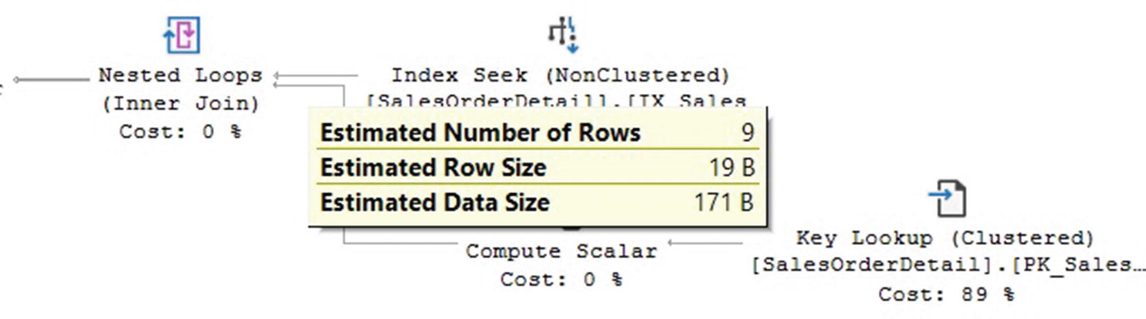
Plan showing estimated number of rows
You can also see the estimated number of rows in the final execution plan, along with the actual number of rows.
Although sys.stats has the benefit that it can be used programmatically to find the stats_id, for a single request, you would have to run it manually. For example, in my system, I can see that the statistic IX_SalesOrderDetail_ProductID has stats_id value of 3.

Estimated number of rows using average_range_rows
Plan Caching
Once an execution plan is generated by the SQL Server query optimizer, it can be stored in memory to be reused as many times as needed if the same query is executed again. Since query optimization is a very expensive operation in terms of time and system resources, reusing a query plan as much as possible can greatly enhance the performance of your databases. Plans are stored in a part of the memory called the plan cache (which was previously known as the procedure cache), and they are only removed in a few cases such as when there is SQL Server memory pressure, when some configuration changes are performed either at the instance or database level, or when certain statements (like DBCC FREEPROCACHE) are executed. The plan cache is part of the memory you allocate to SQL Server along with the buffer pool, which is used to store database pages.

SQL Server compilation and recompilation process
In order to use an existing execution plan, some validations are still needed. The SQL Server compilation and recompilation process is shown in Figure 1-17, where you can notice that even after a plan for a batch is found in the plan cache, it is still validated for correctness-related reasons. This means that a plan that was used even a moment ago may no longer be valid after some database changes, for example, a change on a column or an index. Obviously, if the plan is no longer valid, a new one has to be generated by the query optimizer, and a recompilation will occur.
After a plan has been found valid for correctness-related reasons, it is next validated for optimality or performance-related reasons. A typical case in this validation is the presence of new or outdated statistics. Once again, if a plan fails this validation, the batch will be sent for optimization, and a new plan will be generated. In addition, if statistics are out of date, they will need to be automatically updated first if default SQL Server settings are used. If automatic update of statistics is disabled, which is rarely recommended, then this update will be skipped. If asynchronous update of statistics is configured, the query optimizer will use existing statistics that would be updated asynchronously later and most likely available for the next optimization that may require them. In any of these cases, a new generated plan may be kept in the plan cache so it can be reused again. It is worth noting here that it is possible that the old and the new plan may be the same or very similar if not enough changes were done in the system and the optimizer takes the same decisions as earlier. But then again this is a validation that is required for correctness and performance-related reasons.
I have emphasized so far that reusing a plan is desired in order to avoid expensive optimization time and cost resources. However, even after passing the optimality validation indicated earlier, there may be cases when reusing a plan may not help performance wise, and requesting a new plan would instead be a better choice. This is particularly true in the case of parameter-sensitive queries where, because of skewed or uneven data distribution, reusing a plan created with one parameter may not be adequate for the same query with a different parameter. This is sometimes referred to as the parameter sniffing problem, although, in reality, parameter sniffing is a performance optimization that the query optimizer uses to generate a plan especially tailored for the particular parameter values initially passed in. It is the fact that this does not work fine all the time that has given parameter sniffing its bad reputation.
Query Execution
As mentioned in the previous section, the query optimizer assembles a plan choosing from a collection of operations available on the execution engine, and the resulting plan is used by the query processor to retrieve the desired data from the database. In this section, I will describe the most common query operators, also called iterators, and the most common operations that you will see in execution plans.
Operators
Open(): Causes an operator to initialize itself and set up any required data structures
GetRow(): Requests a row from the operator
Close(): Performs some cleanup operations and shuts itself down
The execution of a query plan consists in calling Open() on the operator at the root of the tree, then calling GetRow() repeatedly until it returns false, and finally calling Close(). The operator at the root of the tree will in turn call the same methods on each of its child operators, and these will do the same on their child operators, and so on. For example, an operator can request rows from their child operators by calling their GetRow() method . This also means that the execution of a plan starts from left to right, if we are looking at a graphical execution plan in SQL Server Management Studio.
Since the GetRow() method produces just one row at a time, the actual number of rows displayed in the query plan is usually the number of times the method was called on a specific operator, plus an additional call to GetRow() to indicate the end of the result set. At the leaf of the execution plan trees, there are usually data access operators that actually retrieve data from the storage engine accessing structures like tables, indexes, or heaps. Although the execution of a plan starts from left to right, data flows from right to left. As the rows flow from right to left, additional operations are performed on them including aggregations, sorting, filtering, joins, and so on.
It is worth noting that processing one row at a time is the traditional query processing method used by SQL Server and that a new approach introduced with columnstore indexes can process a batch of rows at a time. Columnstore indexes were introduced with SQL Server 2012 and will be covered in detail in Chapter 7.
Live Query Statistics, a query troubleshooting feature introduced with SQL Server 2016, can be used to view a live query plan while the query is still in execution, allowing you to see query plan information in real time without the need to wait for the query to complete. Since the data required for this feature is also available in the SQL Server 2014 database engine, it can also work in that version if you are using SQL Server 2016 Management Studio. Live Query Statistics is covered in Chapter 6.
Although all iterators require some small fixed amount of memory to perform its operations (store state, perform calculations, etc.), some operators require additional memory and are called memory-consuming operators. On these operators, which include sort, hash join, and hash aggregation, the amount of memory required is generally proportional to the number of estimated rows to be processed. More details on memory required by operators will be discussed later in this chapter. The query processor implements a large number of operators that you can find at https://msdn.microsoft.com/en-us/library/ms191158. The following section includes an overview of the most used query operations .
Data Access Operators
Data Access Operators
Structure | Scan | Seek |
|---|---|---|
Heap | Table scan | |
Clustered index | Clustered index scan | Clustered index seek |
Nonclustered index | Index scan | Index seek |
An additional operation that is not listed in Table 1-3, as it is not an operation per se, is a bookmark lookup. There might be cases when SQL Server needs to use a nonclustered index to quickly find a row in a table, but the index alone does not cover all the columns required by the query. In this case, the query processor would use a bookmark lookup, which in reality is a nonclustered index seek plus a clustered index seek (or a nonclustered index seek plus a RID lookup in the case of a heap). Graphical plans will show key lookup or RID lookup operators although text and XML plans would show the operations I have just described with a lookup keyword with the seek operation on the base table.
Newer versions of SQL Server include additional features that use structures like memory-optimized tables or columnstore indexes that have their own data access operations, which also include scan and seeks . Memory-optimized tables and columnstore indexes will be covered in Chapter 7.
Aggregations
An aggregation is an operation where the values of multiple rows are grouped together to form a single value of more significant meaning or measurement. The result of an aggregation can be a single value, such as the average salary in a company, or it can be a per-group value, such as the average salary by department. The query processor has two operators to implement aggregations, stream aggregate and hash aggregate, which can be used to solve queries with aggregation functions such as AVG or SUM or the GROUP BY or DISTINCT clauses.
Stream aggregate is used in queries with an aggregation function (like AVG or SUM) and no GROUP BY clause, and they always return a single value. Stream aggregate can also be used with GROUP BY queries with larger data sets when the data provided is already sorted by the GROUP BY clause predicate, for example, by using an index. A hash aggregate could be used for larger tables where data is not sorted, there is no need to sort it, and only a few groups are estimated. Finally, a query using the DISTINCT keyword can be implemented by a stream aggregate, a hash aggregate, or a distinct sort operator. The main difference with the distinct sort operator is that it both removes duplicates and sorts its input if no index is available. A query using the DISTINCT keyword can be rewritten as using the GROUP BY clause, and they will generate the same plan.
We have seen so far that there might be operators that require the data to be already ordered. This is the case for the stream aggregate and also the case for the merge join, which we will see next. The query optimizer may employ an existing index, or it may explicitly introduce a sort operator to provide sorted data. In some other cases, data will be sorted by using hash algorithms, which is the case of the hash aggregation shown in this section, and the hash join, covered next. Both sorting and hashing are stop-and-go or blocking operations as they cannot produce any rows until they have consumed all their input (or at least the build input in the case of the hash join). As shown in the “Memory Grants” section later, incorrect estimation of the required memory can lead to performance problems.
Joins
A join is an operation that combines records from two tables based on some common information that usually is one or more columns defined as a join predicate. Since a join processes only two tables at a time, a query requesting data from n tables must be executed as a sequence of n – 1 joins. SQL Server uses three physical join operators to implement logical joins: nested loops join, merge join, and hash join. The best join algorithm depends on the specific scenario, and, as such, no algorithm is better than the others. Let’s quickly review how these three algorithms work and what their cost is.
Nested Loops Join
In the nested loops join algorithm, the operator for the outer input (shown at the top on a graphical plan) will be executed only once, while the operator for the inner input will be executed once for every row that qualifies for the join predicate. The cost of this algorithm is the size of the outer input multiplied by the size of the inner input. A nested loops join is more appropriate when the outer input of the join is small and the inner input has an index on the join key. The nested loops join can be especially effective when the inner input is potentially large, there is a supporting index, and only a few rows qualify for the join predicate, which also means only a few rows in the outer input will be searched.
Merge Join
A merge join requires an equality operator on the join predicate and its inputs sorted on this predicate. In this join algorithm, both inputs are executed only once, so its cost is the sum of reading both inputs. The query processor is not likely to choose a merge join if the inputs are not already sorted, although there may be cases, depending on the estimated cost, when it may decide to sort one or even both inputs. The merge join algorithm works by simultaneously reading and comparing a row from each input, returning the matching rows until one or both of the tables are completed.
Hash Join
Similar to the merge join, a hash join requires a join predicate with an equality operator, and both inputs are executed only once. However, unlike the merge join, it does not require its inputs to be sorted. A hash join works by creating a hash table in memory, called the build input. The second table, called the probe input, will be read and compared to the hash table, returning the rows that match. A performance problem that may occur with hash joins is a bad estimation of the memory required for the hash table, in which case there might not be enough memory allocated and may require SQL Server to use a workfile in tempdb. The query optimizer is likely to choose a hash join for large inputs. As with merge joins, the cost of a hash join is the sum of reading both inputs.
Parallelism
Parallelism is a mechanism used by SQL Server to execute parts of a query on multiple different processors simultaneously and then combine the output at the end to get the correct result. In order for the query processor to consider parallel plans, a SQL Server instance must have access to at least two processors or cores, or a hyperthreaded configuration, and both the affinity mask and the max degree of parallelism configuration options must allow the use of at least two processors.
The max degree of parallelism advanced configuration option can be used to limit the number of processors that can be used in parallel plans. A default value of 0 allows all available processors to be used in parallelism. On the other side, the affinity mask configuration option indicates which processors are eligible to run SQL Server threads. The default value of 0 means that all the processors can be used. SQL Server will only consider parallel plans for queries whose serial plans estimated cost exceeds the configured cost threshold for parallelism, whose default value is 5. This basically means that if you have the proper hardware, a SQL Server default configuration value would allow parallelism with no additional changes.
Parallelism in SQL Server is implemented by the parallelism operator, also known as the exchange operator, which implements the Distribute Streams, Gather Streams, and Repartition Streams logical operations.
Parallelism in SQL Server works by splitting a task among two or more instances of the same operator, each instance running in its own scheduler. For example, if a query is required to count the number of records on a small table, a single stream aggregate operator may be just enough to perform the task. But if the query is requested to count the number of records in a very large table, SQL Server may use two or more stream aggregate operators, which will run in parallel, and each will be assigned to count the number of records of a part of the table. Each stream aggregate operator will perform part of the work and would run in a different scheduler.
Updates
Update operations in SQL Server also need to be optimized so they can be executed as quickly as possible and are sometimes more complicated than SELECT queries as they not only need to find the data to update but may also need to update existing indexes, execute triggers, and reinforce existing referential integrity or check constraints.
Update operations are performed in two steps, which can be summarized as a read section followed by the requested update section. The first step determines which records will be updated and the details of the changes to apply and will read the data to be updated just like any other SELECT statement. For INSERT statements, this includes the values to be inserted, and for DELETE statements, the keys of the records to be deleted, which could be the clustering keys for clustered indexes or the RIDs for heaps. For UPDATE statements, a combination of both the keys of the records to be updated and the values to be updated is needed. In the second step, the update operations are performed, including updating indexes, validating constraints, and executing triggers, if required. The update operation will fail and roll back if it violates any constraint.
Memory Grants
Although every query submitted to SQL Server requires some memory, sorting and hashing operations require significant larger amounts of memory, which, in some cases, can contribute to performance problems. Different from the buffer cache, which keeps data pages in memory, a memory grant is a part of the server memory used to store temporary row data while a query is performing sorting and hashing operations, and it is only required for the duration of the query. This memory is required to store the rows to be sorted or to build the hash tables used by hash join and hash aggregate operators. In rare cases, a memory grant may also be required for parallel query plans with multiple range scans.
- a.
A system running multiple queries requiring sorting or hashing operations may not have enough memory available, requiring one or more queries to wait.
- b.
A plan underestimating the required memory could lead to additional data processing or to the query operator to use disk (spilling).
In the second case , usually due to bad cardinality estimations, the query optimizer may have underestimated the amount of memory required for the query and the sort operations, or the build inputs of the hash operations do not fit into the available memory. You can use the sort_warning, hash_warning, and exchange_spill extended events (or the Sort Warning, Hash Warning, and Exchange Spill trace event classes) to monitor the cases where these performance problems may be happening in your database.
The resource semaphore process is responsible for reserving and allocating memory to incoming queries. When enough memory is available in the system, the resource semaphore will grant the requested memory to queries in a first-in, first-out (FIFO) basis so they can start execution. If not enough memory is available, the resource semaphore will place the current query in a waiting queue. As memory becomes available, the resource semaphore will wake up queries in the waiting queue and will grant the requested memory so they can start executing. Additional information about the resource semaphore can be shown using the sys.dm_exec_query_resource_semaphores, which, in addition to the regular resource semaphore described here, describes a small-query resource semaphore. The small-query resource semaphore takes care of queries that requested memory grant less than 5 MB and query cost less than three cost units. The small-query resource semaphore helps improve response time for small queries that are expected to execute very fast.
Related wait type RESOURCE_SEMAPHORE_QUERY_COMPILE indicates excessive concurrent query compiles. RESOURCE_SEMAPHORE_MUTEX shows waits for a thread reservation when running a query, but it also occurs when synchronizing query compile and memory grant requests. More details on waits will be covered in Chapter 5.
Finally, the memory grant feedback, a feature introduced with SQL Server 2017, was designed to help with these situations by recalculating the memory required by a query and updating it in the cached query plan. The memory grant feedback comes in two flavors, batch mode and row mode , and it is covered in more detail in Chapter 10.
Locks and Latches
Latches are short-term lightweight synchronization primitives used to protect memory structures for concurrent access. They must be acquired before data can be read from or written to a page in the buffer pool depending on the access mode preventing other threads from looking at incorrect data. Latches are SQL Server internal control mechanisms and are only held for the duration of the physical operation on the memory structure. Performance problems relating to latch contention may happen when multiple threads try to acquire incompatible latches on the same memory structure.
- a.
PAGELATCH_: They are called buffer latches as they are used for pages in the buffer pool. Pages are the fundamental unit of data storage in SQL Server, and their size is 8 KB. Pages include data and index pages for user objects along with pages that manage allocations such as the IAM (Index Allocation Map), PFS (Page Free Space), GAM (Shared Global Allocation Map), and SGAM (Shared Global Allocation Map) pages.
- b.
PAGEIOLATCH: Similar to the previous type of latch, they are also latches for pages, but these are used in the case where a page is not yet loaded in the buffer pool and needs to be accessed from disk. They are often referred to as I/O latches.
- c.
LATCH_ and TRAN_MARKLATCH: These are used for internal memory structures other than buffer pool pages and so are simply known as nonbuffer latches.
The sys.dm_os_latch_stats DMV can be used to return information about all latch waits in the system and is organized by classes. All the buffer latch waits are included in the BUFFER latch_ class, and all remaining classes are nonbuffer latches. Since latch contention in allocation pages is a common problem on the tempdb database, this topic will be explained in more detail in Chapter 4, which covers tempdb troubleshooting and configuration.
Locking, on the other hand, is a mechanism used by SQL Server to synchronize access to the same data by multiple users at the same time. There are several ways to get information about the current locking activity in SQL Server such as using the sys.dm_tran_locks DMV. The main difference between locks and latches is that latches are used to guarantee consistency of memory structures and that they are held for the duration of the physical operation on this memory structure. Locks are used to guarantee the consistency of a transaction and are controlled by the developer, for example, by the use of transaction isolation levels.
SQL Server also uses similar structures called superlatches (sometimes called sublatches) to provide increased performance in highly concurrent workloads. SQL Server will dynamically promote a latch into a superlatch or demote it as needed.
Waits and contention on locks and latches are inevitable as part of the normal operation on a busy SQL Server instance. The challenge is to identify when these waits are excessive and may create a performance problem. Waits for any SQL Server resource are always recorded and available as inside the SQL Server code it is required to indicate what resource the code is waiting for. Waits for locks and latches are covered in great detail in Chapter 5.
Summary
This chapter covered how the SQL Server database engine works and explained everything happening in the system from the moment a connection is made to a database until a query is executed and the results are returned to the client. TDS was introduced as an application-level protocol that facilitates the interaction between clients and SQL Server. We also saw how operating system services are general-purpose services and many times inappropriate for database engine needs as they do not scale well.
We covered how the query processor works and how the query optimizer assembles an efficient execution plan using the operations provided by the database engine. With a large number of operators available in SQL Server, we covered the most used operations as well, including operators for data access, aggregations, joins, updates, and parallelism. Memory grants and locks and latches were discussed as well as many performance problems that require a basic understanding of how they work.
This introductory chapter didn’t include newer database engine structures such as columnstore indexes or memory-optimized tables, which are totally new technologies and require an entire chapter. Chapter 7 is dedicated to those in-memory technologies.