
APPENDIX A
Selected Distributions
This appendix describes a partial set of useful probability distributions, suggestions for when to use them, and how to replicate them for simulations in Excel. There is also a spreadsheet on this book’s website with all of these distributions already set up in Excel:
Distribution Name: Triangular
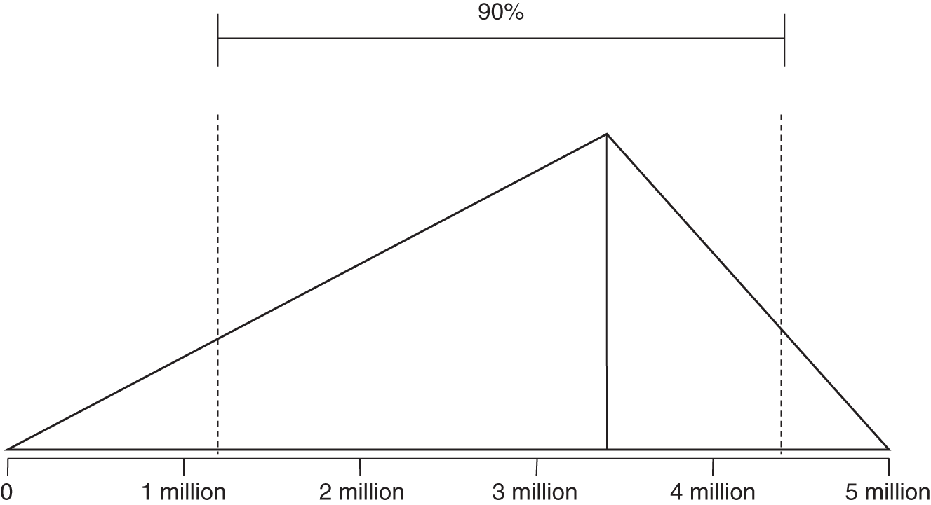
FIGURE A.1 Triangular distribution
Parameters:
- UB (Upper bound);
- LB (Lower bound);
- Mode—this may be any value between UB and LB.
Note that UB and LB are absolute outer limits—a 100% CI.
For a triangular distribution, the UB and LB represent absolute limits. There is no chance that a value could be generated outside of these bounds. In addition to the UB and LB, this distribution also has a mode that can vary to any value between the UB and LB. This is sometimes useful as a substitute for a lognormal, when you want to set absolute limits on what the values can be but you want to skew the output in a way similar to a lognormal. It is useful in any situation where you know of absolute limits but the most likely value might not be in the middle, as in the normal distribution.
- When to use: When you want control over where the most likely value is compared to the range, and when the range has absolute limits.
- Examples: Number of records lost if you think the most likely number is near the top of the range and yet you have a finite number of records you know cannot be exceeded.
- Excel formula:
Note: we use the Excel “Let” function here because the formula assumes the same value from the rand() function will be reused. If we used a separate rand() function each of the times a random number is called in this formula, four different values would be generated and this function would not produce the correct triangular distribution. In the downloadable spreadsheet, we use the HDR PRNG, which will always produce the same pseudorandom value given the same counter values.
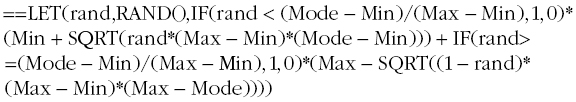
Distribution Name: Binary
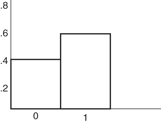
FIGURE A.2 Binary distribution
Parameters:
- P (Event probability)
Note that P is between 0 and 1. It represents how frequently the simulation will randomly produce an event.
Unlike the other distributions mentioned here, a discrete binary distribution (also known as a Bernoulli distribution) generates just two possible outcomes: success or failure. The probability of success is p and the probability of failure is q = (1 − p). For example, if success means to flip a fair coin heads up, the probability of success is p = 0.5, and the probability of failure is q = (1 − 0.5) = 0.5.
- When to use: This is used in either/or situations—something either happens or it doesn't.
- Example: The occurrence of a data breach in a given period of time.
- Excel formula: =if(rand() < P,1,0)
- Mean: =P.
Distribution Name: Normal
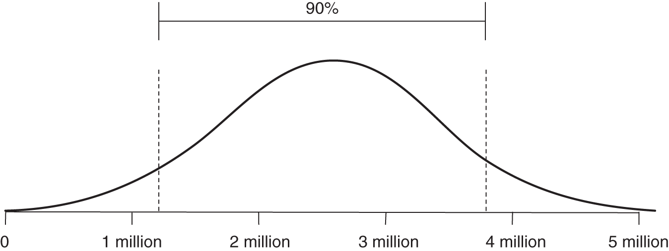
FIGURE A.3 Normal distribution
Parameters:
- UB (Upper bound)
- LB (Lower bound)
Note that LB and UB in the Excel formula below represent a 90% CI. There is a 5% chance of being above the UB and a 5% chance of being below the LB.
A normal (or Gaussian) distribution is a bell‐shaped curve that is symmetrically distributed about the mean.
- Many natural phenomena follow this distribution but in some applications it will underestimate the probability of extreme events.
- Empirical rule: Nearly all data points (99.7%) will lie within three standard deviations of the mean.
- When to use: When there is equal probability of observing a result above or below the mean.
- Examples: Test scores, travel time.
- Excel formula: =norm.inv(rand(),(UB + LB)/2,(UB‐LB)/3.29)
- Mean: =((UB + LB)/2)
Distribution Name: Lognormal
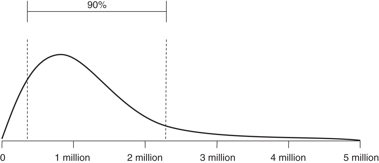
FIGURE A.4 Lognormal distribution
Parameters:
- UB (Upper bound)
- LB (Lower bound)
Note that LB and UB in the Excel formula below represent a 90% CI. There is a 5% chance of being above the UB and a 5% chance of being below the LB.
The lognormal distribution is an often preferred alternative to the normal distribution when a sample can only take positive values. Consider the expected future value of a stock price. In the equation S1 = S0er, S1 is the future stock price, S0 is the present stock price, and r is the (continuously compounded) expected rate of return (e is the base of the natural log, 2.71828…). The expected rate of return follows a normal distribution and may very well take a negative value. The future price of a stock, however, is bounded at zero. By taking the exponent of the normally distributed expected rate of return, we will generate a lognormal distribution where a negative rate may have an adverse effect on the future stock price, without ever leading the stock price below the zero bound. It also allows for the possibility of extreme values on the upper end and, therefore, may fit some phenomena better than a normal.
- When to use: To model positive values that are primarily moderate in scope but have potential for rare extreme events.
- Examples: Losses incurred by a cyberattack, the cost of a project.
- Excel formula: =lognorm.inv(rand(),(ln(UB) + ln(LB))/2, (ln(UB)‐ ln(LB))/3.29)
- Mean: = ((ln(UB)+ln(LB))/2)
Distribution Name: Beta
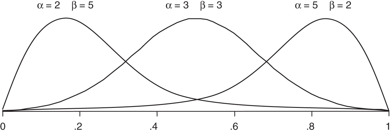
FIGURE A.5 Beta distribution
Parameters:
- Alpha (1 + Number of hits)
- Beta (1 + Number of misses)
Beta distributions are extremely versatile. They can be used to generate values between 0 and 1 but where some values are more likely than others. This result can also be used in other formulas to generate any range of values you like. They are particularly useful when modeling the frequency of an event, especially when the frequency is estimated based on random samples of a population or historical observations. In this distribution it is not quite as easy as in other distributions to determine the parameters based only on upper and lower bounds. The only solution is iteratively trying different alpha and beta values until you get the 90% CI you want. If alpha and beta are each greater than 1 and equal to each other, then it will be symmetrical, where values near 0.5 are the most likely and less likely further away from 0.5. The larger you make both alpha and beta, the narrower the distribution. If you make alpha larger than beta, the distribution will skew to the left, and if you make beta larger, it skews to the right.
To test alpha and beta, just check the UB and LB of a stated 90% CI by computing the fifth and ninety‐fifth percentile values. That is betainv(.05,alpha,beta) and betainv(.95,alpha,beta). You can check that the mean and mode are what you expect by computing the following: mean = alpha/(alpha+beta), and mode (the most likely value) is mode = (alpha‐1)/(alpha+beta‐2). Or you can just use the spreadsheet at www.howtomeasureanything.com/cybersecurity to test the bounds, means, and modes from a given alpha and beta to get good approximations of what you are estimating.
- When to use: Any situation that can be characterized as a set of “hits” and “misses.” For each hit, increase alpha by 1. For each miss, increase beta by 1.
- Examples: Frequency of an event (such as a data breach) when the frequency is less than 1 per time unit (e.g., year), proportion of employees following a security procedure correctly.
- Excel formula: =betainv(rand(),alpha,beta)
- Mean: =(alpha/(alpha + beta))
Distribution Name: Power Law
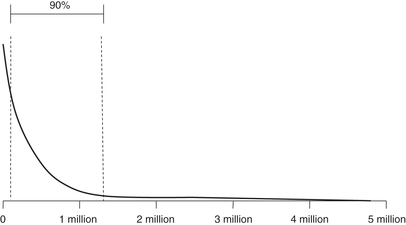
FIGURE A.6 Power law distribution
Parameters:
- Alpha (Shape parameter)
- Theta (Location parameter)
The power law is a useful distribution for describing phenomena with extreme, catastrophic possibilities—even more than lognormal. For events such as forest fires, the vast majority of occurrences are limited to an acre or less in scope. On rare occasions, however, a forest fire may spread over hundreds of acres. The “fat tail” of the power law distribution allows us to acknowledge the common small event, while still accounting for more extreme possibilities.
- When to use: When you want to make sure that catastrophic events, while rare, will be given nontrivial probabilities.
- Examples: Phenomena such as earthquakes, power outages, epidemics, and other types of “cascade failures” have this property.
- Excel formula: =(theta/rand())^alpha
- Mean: =(alpha*theta/(alpha‐1))