9

Analysis of Operational Results

Learning Objectives By the end of this chapter, you should be able to: • List the three kinds of costs. • Explain the term break-even point. • List three uses of break-even analysis. • Define the term contribution margin. • Identify the five factors that influence cost-volume-profit analysis.

INTRODUCTION

One’s objective in managing a business is described simply in this way: to assure that the benefits achieved exceed the sacrifices made. Managers are constantly faced with decisions about selling prices, variable and fixed costs, choice of product lines, market strategy, utilization of production facilities, and acquisition and employment of economic resources in pursuit of some goal or objective. The bases for financial planning and control include cost-behavior analysis, evaluation of cost-volume-profit relationships, and flexible budgeting. Flexible budgeting allows the effect of changes in anticipated volume to be taken into account and involves a series of budgets for varying levels of activity. Many managers are interested in cost behavior, cost control, and cost measurement. This chapter presents information that will aid in their planning and control.

COST BEHAVIOR

The first basis for planning and control, cost behavior, refers to the degree of responsiveness a cost has at various activity levels. There are fixed costs, variable costs, and mixed costs.

Fixed Costs

Fixed costs remain unchanged within a relevant range of activity. If straight-line depreciation is used for fixed-asset write-off, the cost is fixed and unchanging for a specific, short time period. Reference to a particular time period is essential to the concept of a fixed cost because all costs tend to be variable over a long period of time. For consistency, the time frame used in this text is one year.

Although the fixed cost will have the same total, the unit rate changes inversely with volume. For example, assume annual depreciation of $100,000, using the straight-line method. This amount is charged as a cost, regardless of the level of production or sales. At the 100,000-unit level of production, the depreciation rate per unit is one dollar. If 200,000 units were produced, the rate would reduce to 50 cents per unit. Since the fixed cost depends on a particular volume, these amounts will remain constant within a workable range. Supervisors’ salaries provide a good illustration. A supervisor’s salary is fixed, regardless of whether the group of people he or she supervises consists of 20 or 40 people (or any number in between).

Variable Costs

Variable costs, in total, change in direct proportion to an activity level. Total variable costs of a particular cost object (something that you are tracking the cost of) increase with increases in the volume level related activity and decrease with decreases in the volume level of the related activity. For instance, the total cost of raw material used in production varies in relation to the number of units produced. Thus, if a unit of material costs $5, this rate will not change, regardless of the number of units used in production; but the total cost increases directly with the number of material units used in production.

Mixed Costs

Mixed costs are a hybrid cost—part fixed and part variable. For example, a cell phone bill could be a mixed cost if it has a fixed monthly fee plus a rate per minute of usage. Operating company vehicles is a classic example of a mixed cost involving certain fixed costs such as annual insurance and variable costs such as changing fuel prices and differing amounts of use from one month to another.

The algebraic formula for a mixed cost is y = a + bx, where:

y is the total cost

a is the fixed cost per period

b is the variable rate per unit of activity

and x is the number of units of activity

For example, the annual expense of operating a truck might be found using the following formula:

$5,000 + .30x

Where x is the number of miles driven (the activity).

If the truck is driven 20,000 miles in a particular year, the cost would be:

$5,000 + .3(20,000) = $11,000

COST-VOLUME-PROFIT ANALYSIS

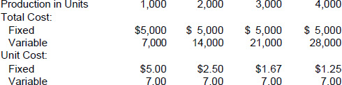
The cost-volume-profit (CVP) analysis in this chapter covers only variable and fixed expenses. Exhibit 9–1 shows the relationship of total costs to unit costs at various levels of production. If the total fixed cost remains the same, the cost per unit decreases as volume increases. The total variable cost increases directly with an increase in production, but the rate of increase is constant.

Five important factors influence cost-volume-profit analysis. They are:

1. Fixed costs

2. Variable costs

3. Selling prices of products

4. Volume of sales or level of sales activity

5. Mixture of the types of products sold

All of these factors must be weighed by management when engaging in profit planning and cost control.

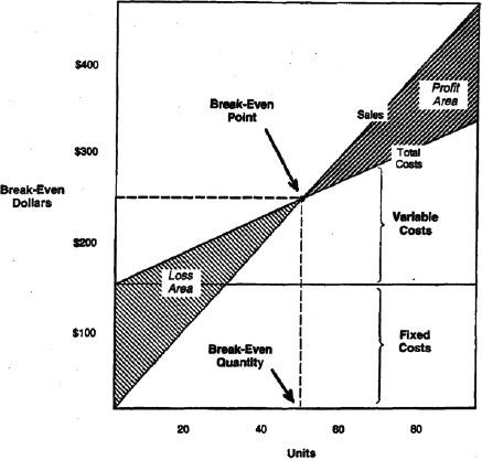
Break-Even Point

The study of cost-volume-profit analysis, often called break-even analysis, stresses the relationship among the five elements listed above. The break-even point is the point where the volume of sales or level of operations produces neither a net income nor a net loss. In other words, the break-even point is where revenues will just cover costs. This point can be found mathematically or by preparing a graph. Whichever method is used, all costs are separated into fixed and variable categories.

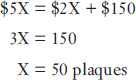
Working with an example is the best way to understand the break-even point calculation. For example, John Smith is a college student who earns his tuition by doing odd jobs and taking on small business ventures. He plans on selling historical plaques during a Fourth of July picnic. He purchases the plaques for $2 each, retaining the option to return all unsold items. The rental of his booth costs $150. If the plaques sold for $5 each, how many would John have to sell in order to break even? (Ignore income taxes.)

In determining the break-even point using a mathematical computation, you must understand the most elementary formula for computing a break-even point:

Break-Even Sales = Variable Cost + Fixed Cost

If you let X = sales at break-even (units of dollars), you can plug John Smith’s data into the equation as follows:

Proof:

Sales = 50 plaques @ $5 each = $250

Cost and Expenses—Variable:

50 Plaques @ $2 each = $100

Fixed:

What would John’s profit be if he sold 51 plaques? Quite often, people assume the answer is $5. But calculation is necessary to be sure.

Sales = 51 plaques @ $5 each = $255

Cost and Expenses—Variable:

51 Plaques @ $2 each = $102

Fixed:

The cost of the plaques fluctuates directly with the quantity purchased—a variable cost. Fixed cost is recovered with the sale of the first 50 plaques. Thereafter, the sale of each plaque contributes to profit, after covering the variable cost per unit.

By expanding on the basic formula, it can be determined how many plaques must be sold to earn a particular profit. Suppose John Smith wanted to earn $75 for the period of time he spends in his booth. The formula would be expanded to solve for the $75 profit as follows:

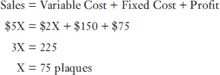
Proof:

Sales = 75 plaques @ $5 = $375

Cost and Expenses—Variable:

75 plaques @ $2 = $150

Fixed:

THE GRAPHIC PRESENTATION OF BREAK-EVEN

A break-even point graph can be used to determine the dollar or unit amount at which there will be no profit or loss. Exhibit 9–2 plots John Smith’s information. Although the graph is not accurate decimally, it is adequate for the limited range used here.

The sales and total expense lines cannot be plotted ad infinitum with the hope of maximizing profit to the nth degree. A saturation point will be reached where sales begin to drop or where both fixed and variable costs begin to increase. Here the lines on the graph cross each other again; the area beyond the second juncture is a loss area.

Sales may begin to slow down because there are fewer buyers in the market who want to purchase. On the other hand, costs and expenses may begin to climb because the scarcity of material may cause prices to rise, or because the labor supply may have been reduced to a level that necessitates offering a monetary incentive to obtain the required work force.

USING BREAK-EVEN ANALYSIS

The break-even point is helpful to management for forecasting, evaluating managerial efficiency, and decision making. As a forecasting tool, the break-even point can aid in determining the following:

• The requirements of the sales department that justify a proposed investment in plant expansion

• The effect of increases and decreases in sales volume

• The probable cost per unit of manufactured goods at various production levels

• The evaluation of changes in production methods

• The planning of profit objectives

Managerial efficiency may be evaluated by comparing actual break-even results with predetermined levels. If properly considered by management, the break-even point and the analysis of cost-volume-profit can be valuable tools when used in conjunction with the analysis of sales mix and the conversion of variable costs to fixed costs. For example, management may be considering a capital expenditure in order to automate equipment. This decision would shift some costs from variable to fixed, thus changing the break-even point.

CONTRIBUTION MARGIN

The contribution margin is most easily defined as the difference between sales and variable costs. The excess of sales over variable costs can be used to contribute toward meeting fixed costs and achieving a profit for the period. A comparison of contribution margin and the traditional income statement, and how they each arrive at net income, is shown in Exhibit 9–3. The contribution margin is employed by management because costs are classified by behavior (variable or fixed) rather than by function (production, sales, or administration). It should be noted, however, that contribution margin is not the same as gross margin or gross profit, which is computed in the traditional format.

Once again, the John Smith venture can illustrate the contribution margin approach.

Sale price per plaque ($5) − Variable cost per plaque ($2) = Unit Contribution Margin ($3)

Since the contribution margin of $3 will cover fixed costs, the next question is: How many units must be sold to cover the $150 rental with no anticipated profit?

The calculation for the break-even point in dollars, using the contribution margin, requires a contribution percentage. In Smith’s venture, 60 percent ($3 out of $5) of the total selling price is contributed toward fixed costs and profit. Since profit does not enter into the calculation of the break-even point, the dollars of sales needed are:

The contribution margin computation for the $75 profit desired by Smith is:

Fixed Costs ($150) + Desired Profit ($75) = $375 Contribution Margin Ratio (0.60)

Advantages of Cost-Volume-Profit Analysis

Cost behavior patterns offer valuable insights into planning and controlling long-term and short-term operations. It is obligatory that management become fully cognizant of cost-volume-profit analysis. Management’s duty is to discover the combination of fixed and variable costs that will be most beneficial to the company. A firm that has a large and highly salaried sales force (fixed cost) may discover through the contribution margin that, after deducting variable costs from sales, there is an insufficient remainder to contribute toward fixed costs and profit. It may be less costly for the company to employ manufacturers’ representatives and compensate them using commission, a variable cost. Remuneration would then vary directly with sales.

When management sets a profit goal for a specific period of time (annual, semi-annual, quarterly), it is easy to compute the number of units that must be sold in order to reach the goal; this is done simply by dividing the fixed costs plus desired profit by the contribution margin per unit. When the contribution margin is low, a large increase in sales must occur in order to produce a significant increase in profit. Another look at Exhibit 9–2 reveals that, as sales move beyond the break-even point, the contribution margin ratio increases and thus profits also increase at a faster rate.

The external analyst may be unable to project future break-even points at various sales volumes because he or she does not ordinarily have access to data that are exact enough. Nevertheless, the analyst’s conclusions, although rough at best, are meaningful. The variable costs may be difficult to project, but conclusions on fixed costs should be within the limits of company tolerance. Although shortcomings in cost-volume-profit analysis do exist, and the analysis does require laborious effort, performance evaluation is less difficult given the results of such an analysis.

Limitations of Cost-Volume-Profit Analysis

The function of profit projection is vitally important to financial analysts, but it is not without its shortcomings. Clear assignment of costs to either a fixed or variable category is not always possible. The interpretations of several analysts will probably differ. For example, machinery rent that is based on units produced can be classified as a variable cost when production fluctuates. However, if production is steady for a period of time beyond the predetermined range, some analysts may think of the rent as a fixed cost. This differentiation is often difficult for the internal analyst to determine. For the outside analyst, categorization is an almost impossible task if he or she does not possess a considerable amount of internal data.

Direct labor is usually classified as a variable cost. Any change in production volume will have a direct effect on labor in the same direction. If management decides on a temporary shutdown of operations, the effect on the variability of labor cost may not correspond directly. If, for example, the company wishes to retain its highly experienced and skilled personnel during the shutdown period so as not to lose them, the fluctuating nature of direct labor is changed.

Another major weakness of cost-volume-profit analysis as a planning or controlling device occurs in a manufacturing business. The assumption by the analyst that sales and production volumes will always be the same may be valid in theory but not in fact. Business is dynamic, and qualifying a specific cost analysis with the prefatory statement, “other things being equal,” will not necessarily produce a valid result because “other things” will not be equal.

Analysis covering an extended period of time requires a common denominator for all component periods so that data examined will be equivalent. Where costs and prices have changed drastically, adjustments based on current costs and prices produce a more uniform result. Many outside factors must also be kept in mind, such as strikes, lateral and vertical competition, domestic and foreign political developments, and natural disasters.

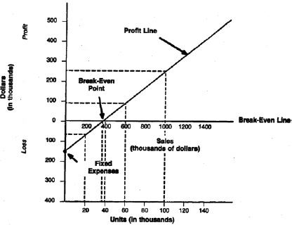
THE PROFIT-VOLUME GRAPH

The profit-volume graph may be used in place of, or along with, the break-even graph. This form is preferred by many managers who are interested mainly in a clearer representation of the effect of volume, since only the net effect of revenue and cost is shown. The graph has a break-even line instead of a break-even point. Exhibit 9–4 shows the vertical axis, calibrated was profit above and loss below the break-even line. The horizontal axis shows units of product.

Plotting a Profit Line

Assume the following data: selling price per unit is $10; variable cost per unit is $6; and fixed expense amounts to $150,000.

The following steps are necessary to plot a profit line on the graph:

1. Fixed expense exists even at zero level of activity; therefore, the fixed-expense point is located on the vertical axis below the break-even line.

2. A point should now be plotted to indicate the amount of profit at a chosen level of sales. The level used in Exhibit 9–4 is 100,000 units, or $1,000,000.

3. Expected profits at this level are:

Sales (100,000 units @ $10 each)	$1,000,000
Less Variable Costs (100,000 × $6)	600,000
Contribution Margin	400,000
Less Fixed Costs	150,000
Net Profit$	250,000

This point is plotted on the graph at the intersection of $1,000,000 of sales and $250,000 of profit. A line is then drawn from this point to connect the fixed-expense point of $150,000 on the vertical axis. The point at which the profit line crosses the horizontal break-even line is the break-even point—37,500 units, or $375,000. The vertical distance between the profit line and the break-even line reflects the expected profit or loss at a specific volume of sales.

The profit-volume graph is often preferred by management because the data are presented more simply than those of a break-even chart. It is a convenient device that quickly outlines the effect on expected profits caused by such changing factors as fixed and variable costs, selling prices, and volume of sales.

The basis of profit planning and control is knowledge of cost behavior. You must know the difference between a fixed and variable cost and how to recognize semi-variable or mixed costs and how they behave with respect to changes in a particular key activity level, such as sales or production. Company cost structures are a complex entanglement of fixed and variable costs, and sometimes it is difficult to sort those costs out. Fixed costs remain unchanged within a relevant range of activity. Variable costs increase with increases in the volume level of related activity and decrease with decreases in the volume level of the related activity, while semi-variable costs are a combination that falls somewhere between fixed and variable cost elements.

Cost-volume-profit (CVP) analysis, which has its origins in break-even analysis, is useful for predicting cost behavior for a company and for planning production levels to produce a desired profit. It is a decision-making tool for management and allows you to ask “what-if ” questions and to see the bottom-line impact of changes in prices, volume, and costs. Management can consider altering any or all of the five factors of CVP when planning. Those factors are fixed costs, variable costs, selling prices, sales volume (units), and the sales mix.

The break-even point can be used either in a formula form or a chart to determine what revenue level is needed to cover all costs exactly. Break-even points are often shown in business plans, as investors and creditors like to see what it will take to cover costs.

Break-even analysis can be modified so that the level of revenue needed to achieve a profit target can be known. Management can set target profit levels and then use the break-even model to determine what volume of sales will be necessary and what level of costs will need to be incurred to meet profit goals.

The contribution margin is another useful tool. It is found on a per unit basis by subtracting variable costs per unit from the price of a product. Total contribution margin is the difference between total revenue (or sales) and variable costs. Knowing the contribution margin allows you to quickly compute break-even and “back solve” for the production levels needed to produce a desired profit.

ANSWERS TO “THINK ABOUT IT...” QUESTIONS FROM THIS CHAPTER

1. 100 units

2. 267 units

3. $10

4. 700 units

5. 771 units