


Application profiling and tuning
In this chapter, we use some of the HPC applications to illustrate how to employ the PEDE and HPCT tools for profiling and tuning.
Usually people try to locate the hotspots of an application and then optimize it. There are some points that are usually considered for an HPC application profiling and tuning, such as the synchronization, load balance, communication overhead and the memory, file I/O issues, along with the real computation effort. Consequently to work on an existing HPC application for optimization, the first step is profiling to recognize the hot spot, Xprofile, or gprof to provide for this function. Then other tools for different profiling and tuning purpose can be utilized, such as the HPCT from IBM.
A hyper HPC program sPPM [S. Anderson et al], which is written by C and Fortran utilizing MPI and OpenMP for parallel programming is described. The contents describe the procedure to locate the hotspot in this program and analyze the possible reason based on the profiling data, followed by possible tuning hints.
The following topics are discussed in this chapter:
7.1 Profiling and tuning hints for sPPM
This section introduces tuning for sPPM.
7.1.1 A glance at the application sPPM
Look for information about the sPPM application at:
http://www.lcse.umn.edu/research/sppm/README.html
The experiment for sPPM occurs based on Power Linux. This program computes a 3-D hydrodynamics problem on a uniform mesh using a simplified version of the PPM (Piecewise Parabolic Method) code.
The coordinates are -1:1 in x and y, and 0:zmax in z, where zmax depends on the overall aspect ratio prescribed. A plane shock traveling up the +z axis encounters a density discontinuity, at which the gas becomes denser. The shock is carefully designed to be simple, but strong, about Mach 5. The gas initially has a density of 0.1 ahead of the shock. At over 5dz at the discontinuity, it changes to 1.0.
This version of sPPM is implemented primarily in Fortran with system-dependent calls in C. All message passing is done with MPI. Only a small set of MPI routines are actually required:
•MPI_Init, MPI_Comm_rank, MPI_Comm_size, MPI_Finalize
•MPI_Wtime, MPI_IRecv, MPI_Isend
•MPI_Wait, MPI_Allreduce, MPI_Request_free
The parallelization strategy within an SMP is based on spawning extra copies of the parent MPI process. This is done with the sproc routine, which is similar but not identical to the standard UNIX fork call. It differs in that sproc causes all static (for example, not stack based) storage to be implicitly shared between processes on a single SMP node. This storage is always declared in Fortran with either SAVE or COMMON.
Synchronization is accomplished by examining shared variables and by use of UNIX System V semaphore calls. (See twiddle.m4 and cstuff.c.) In addition, a fast-vendor supplied implementation of an atomic fetch and add (test_and_add) is used.
7.1.2 Use gprof to view the profiling data
As described in advance, various approaches can be applied to get different types of profiling data. To get the cpu time profiling data of a program, we must compile the source code with -p -pg. After execution, for each MPI task, a gmon.out file is generated, making it possible to use gprof to generate data issuing the command:
-bash-4.1$ gprof ../sppm gmon.out > prof.txt
In this command:
•sppm is the executable
•gmon.out is the raw profiling data
•the prof.txt contains the readable profiling data
Specifically for the sppm application, the output is shown in Figure 7-1 on page 143.
Figure 7-1 The CPU time profiling for sPPM
So from the flat profiling result, the function sppm, difuze and interf took over 80% of the time. Besides, these functions are invoked millions of times, so it is useful if we do optimization for these functions. Because if any slight benefit is brought in, it can be multiplied with millions due to the amount of calls. However it is possible that it is hard to get these functions optimized because for each single call, it only takes few times, which means that these function can be highly optimized already. For the function _vrec_P7, it is impossible to do anything with it because it is a built-in function of the compiler library. Thus it is still worthwhile to look at the functions named as hydyz, hydzy, hydxy, dydyx, hydzz. So let us look further into the call graph profiling data. We describe the details for each function call. See Figure 7-2 on page 144.

Figure 7-2 Detailed call graph
Based on the call graph, we can also ascertain that difuze and interf are called by sppm, and it does not have any further children to call. So it is a good choice to start to optimize the code of difuze and interf. Also some other functions must be noticed. Figure 7-3 gives two of the examples.

Figure 7-3 Detailed call graph for hydyz and dydxy
In addition, tools can help to figure out what is the potential problem in some of the hotspots if it is hard to sort out by inspection of the code. Usually the hotspots are either caused by heavy computation with lots of “load and store” instructions or the communication took plenty of time along with load balance issues. Hence in the later sections, possible causes of the hotspots are analyzed.
7.1.3 Using binary instrumentation for MPI profiling
We presented the general steps about binary instrumentation in the previous chapters. However since it is desired to profile all MPI communications for the program, we choose all of the source code file in the instrumentation view, as shown in Figure 7-4.

Figure 7-4 Instrumentation panel
After the instrumented binary is generated, the default profiling setting is sufficient for information that we need to generate trace files only for the application tasks with the minimum, maximum, and median MPI communication time. This is also true for task zero (people might use task), if task zero is not the task with minimum, maximum, or median MPI communication time. If you need trace files generated for additional tasks, make sure the necessary options under the HPC Toolkit menu are checked during the profiling configuration phase. Refer to Chapter 6, “Parallel Environment Developer Edition tools” on page 95 for the details of each options.

Figure 7-5 Options for MPI profiling
Depending on the number of tasks in your application, make sure that the Maximum trace rank and Limit trace rank are set correctly. If your application executes many MPI function calls, you might need to set the value of Maximum trace events to a higher number than the default 30,000 MPI function calls. Refer to Figure 7-5.
Chapter 6, “Parallel Environment Developer Edition tools” on page 95 explains how to do the launching configuration with an application; therefore, using the same setting, just click Pprofile, and the program runs correctly. Synchronize your project for the generated profiling data. You can now open them with HPCT after you right-click the files. The elapsed cpu time for the MPI function calls is displayed in the summary section. Under that, notice the details of each MPI function call in each source code file and further down to each function that invoked MPI routines. For sPPM, we got the summary data in Figure 7-6.
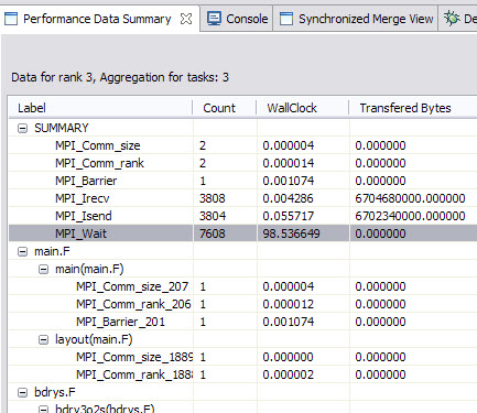
Figure 7-6 sPPM mpi profiling data
We can see the most time consumable MPI routine is MPI_Wait, technically each asychronized MPI_Isend and MPI_Irecv might have one MPI_Wait, so the column of Count illustrates the MPI_Wait has the most frequent invoking, so the wall clock is the highest one. However the communication overhead might not a big issue in this project if comparing with the entire execution time (near 10 minutes). It is still interesting that based on the result shows here, the assumption is the work load on each MPI tasks is not well balanced; otherwise, the MPI_Wait routine only takes a short time. If we look at the MPI trace picture, which can be generated by opening the .mpt file through the mpi trace menu in Figure 7-7 on page 147, we can see that the MPI_wait waits for a longer time with mpi rank 4, 5, 6, 7, which means these rank can get less workload than rank 0, 1, 2, 3. Despite that workload issue, the communication happened many times, it is possible to use depth halo with more boundary data layers to reduce the communication frequency. Another point is it is worthwhile to think about if there is a possible way to reduce the total transferred data size, which can be done with altering the major algorithm.

Figure 7-7 MPI trace picture for sPPM
7.1.4 Use OpenMP profiling to identify if the workload for threads
Because the sPPM code utilizes OpenMP threads for some of the hotspots, we can also profile it to see if there is any load balance issue. Refer to “OpenMP profiling” on page 115 for details about how to get your program instrumented for OpenMP profiling. Here, we choose to profile all of the OpenMP regions listed in Figure 7-8 on page 148. Because of the limitation that it is not supported to profile nested OpenMP parallel region, some of the OpenMP parallel regions cannot get profiling data.

Figure 7-8 Instrument all the OpenMP parallel regions for sPPM
After the execution of the instrumented binary, the OpenMP profiling data was generated. Open the .viz files. The summary data is shown in Figure 7-9.
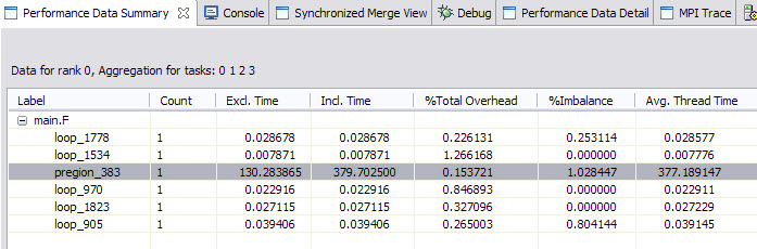
Figure 7-9 OpenMP profiling data
Double-click the most time consumable region. The tool navigates you to which line the code is in the source file. So it is easily located where the OMP issue might be. By further inspecting the code, in this parallel region we have many single and master directives that made the code fragment in serial. So to get better performance, it is necessary to think about how to get those directives less. However based on Figure 7-8 and Figure 7-9, notice that there is no profiling data for the runhyd3.F source code because there are nested OMP regions. As mentioned before, under this circumstance, HPCT does not support OpenMP profiling currently.
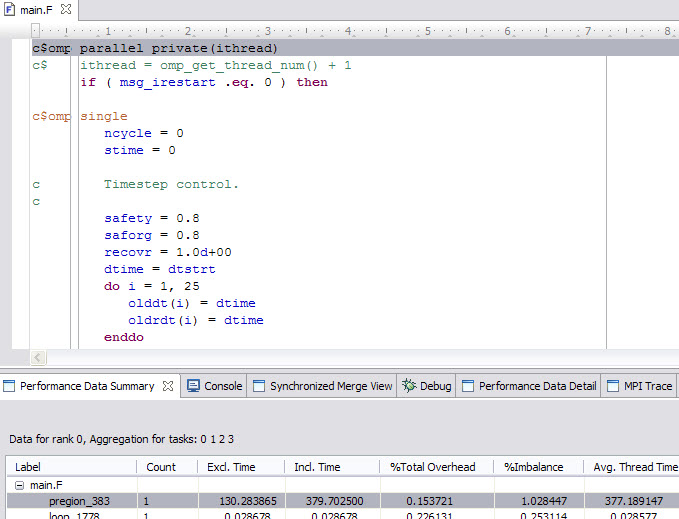
Figure 7-10 hotspot in OpenMP code
In a nut shell, the HPC Toolkit, which is part of the Parallel Environment Developer Edition, can generate profiling data for HPC application developers quickly (Figure 7-10). Based on this profiling data, it is easier to get an idea about how to optimize an existing HPC application without understanding some scientific theory. However there are some other good tools in HPCT with PEDE that are not mentioned here, for example, the I/O profiling, due to sPPM, it does not have heavy I/O operations.
7.2 Profiling and analyzing Gadget 2
Gadget 2 is a freely available application for cosmological simulations widely used in the HPC area, which can be used to address several problems, such as colliding and merging galaxies, dynamics of the gaseous intergalactic medium, or to address star formation and its regulation by feedback processes. Further information about the project along with source code is at:
http://www.mpa-garching.mpg.de/gadget/
This study case takes Gadget2 to:
•Show how to configure a project that requires special build set up.
•Show how to use some basic Eclipse editor features to browse the source code.
•Show how the tools drill-down the application source code looking for performance enhancements opportunities.
Importing Gadget 2 as an existing Makefile application
The Gadget 2 source code was downloaded and uncompressed in the remote Linux on Power cluster node. Next, it was imported in the PEDE Eclipse environment as a synchronized project (see Figure 7-11). The rationale behind our choices are:
•Although the majority of the Gadget’s source code is written in C, we chose to import it as a Synchronized Fortran project because it also contains a small portion of Fortran code and by doing that we ensured that Eclipse handles both Fortran and C/C++ languages properly.
•We imported the project using the empty Makefile project template because Gadget relies on the GNU Makefile build system.
•In one of the steps to import the project, you need to set the connection to the remote node holding the application source code. We managed to create a new connection since there was not one for the PowerLinux node (see Figure 7-12 on page 151).
•We chose --Other Toolchain-- from the Local Toolchain field because PEDE Eclipse was running in a Windows XP notebook, so there was no use in choosing a local toolchain.

Figure 7-11 Creating a synchronized project of Gadget 2

Figure 7-12 Creating a connection with remote PowerLinux cluster node
Configured build settings
The Gadget 2 source code comes from some examples of simulations that are built by different makefiles located in the Gadget2 folder (see Figure 7-13). We chose the Cosmological formation of a cluster of galaxies example for this section, which is built by the Makefile.cluster makefile. So it was needed to change the default settings to properly build the project:
1. Change the default build directory to Gadget2 in the gadget project properties (see Figure 7-14 on page 152).
2. Create a new make target that instructs Eclipse to run make -f Makefile.cluster from the build directory (see Figure 7-15 on page 152). For further information about management of makefile targets, consult the Eclipse help in the menu bar: Help → Help Contents → C/C++ Development User Guide → Tasks → Building projects → Creating a Make target.
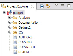
Figure 7-13 Gadget 2 folders hierarchy
Figure 7-14 Changing default build directory

Figure 7-15 Creating a new make target
The project is now built using the cluster target instead of default all. In Figure 7-16 on page 153, the right-column box, Make Target, has an icon for the cluster target where we just double-click it to trigger a fresh build.
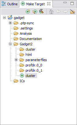
Figure 7-16 New created cluster make target
There is another configuration that many users do not realize is important regarding include paths and preprocessor symbols. If they are not properly set, some features, such as code search and completion, will not work perfectly because the Eclipse C/C++ parse does not understand application source code content completely (Figure 7-17).
Figure 7-17 Gadget 2 preprocessor symbols
More details about how to set Include paths and preprocessor symbols are at the menu: Help → Help Contents → C/C++ Development User Guide → Tasks → Building projects → Adding Include paths and symbols.
Creating a run launcher configuration
The next task was to create a run launcher configuration, which often served as a template for other launch configurations, such as debugger and IBM HPC Toolkit tools.
Our newly created configuration leveraged IBM Parallel Environment (PE) as the execution environment, as shown in Figure 7-18. However, any of the several other execution environments were applicable, and integration is provided by PEDE.

Figure 7-18 Set execution environment
Other tabs in the run launcher configuration were properly fulfilled:
•In the Application tab (Figure 7-19 on page 155): It set the gadget2 executable path.
•In the Arguments tab (Figure 7-20 on page 155): It set the input control file for the
Gadget2 simulation as an argument of the executable. It also changed the default working directory because the input control file makes references to others relative to the Gadget2 folder.
Gadget2 simulation as an argument of the executable. It also changed the default working directory because the input control file makes references to others relative to the Gadget2 folder.
•In the Environment tab (Figure 7-21 on page 156): It was set to a runtime variable that otherwise would fail gadget 2 run. For example, LD_LIBRARY_PATH was exported in runtime because the application depends on third-party shared library and not in a default path.

Figure 7-19 Run launcher configuration: Set application path

Figure 7-20 Run launcher configuration: Set gadget2 arguments

Figure 7-21 Run launcher configuration: Set environment variables
Searching for hot spots using Xprof
We chose to use the Xprof tool (refer to “X Windows Performance Profiler” on page 130) as the first tool toward performance analysis of Gadget 2 because it allows discovery tasks and methods that most impact overall execution time.
The application is built with the required -pg flag, executed with the previous mentioned run configuration to get gprof data files and then loaded into Xprof (see Figure 7-22 on page 157).
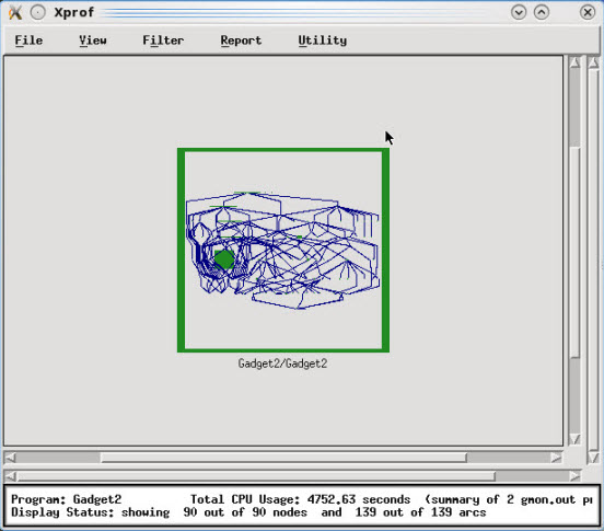
Figure 7-22 Xprof main view
Switching to flat report (menu Report → Flat Profile) enabled us to visualize a rank of methods with the most CPU-intensive on top. Figure 7-23 on page 158 shows that 69.6% of (cumulated) time is spent in a single method named force_treeevaluate_shortrange. The force_treeevaluate_shortrange seemed to be a good candidate for our investigation, but before taking a look at this code we preferred to seek more information.

Figure 7-23 Xprof flat report
After double-clicking force_treeevaluate_shortrange in the flat report, Xprof pointed out the major rectangle in the bottom left of Figure 7-22 on page 157. Graphically, its dimensions represent two measurements:
•The width represents how many times a method was called by its parents.
•The height represents the amount of execution time a method spent in its own code, for example, excluding time spent in its children.
To zoom in the call graph, we applied a filter (menu Filter → uncluster Function) that resulted in Figure 7-24 on page 159.
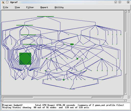
Figure 7-24 Xprof main view with uncluster functions
The force_treeevaluate_shortrange’s rectangle stands out on both width and height proportions. Moreover, Figure 7-25 shows that the total amount of seconds in the self and self+desc fields are equal; therefore, none of the execution time was spent in children methods.

Figure 7-25 force_treeevaluate_shortrange: Sef+desc versus self time
In fact, force_treevaluate_shortrange was an obvious hot spot, but it was also needed to investigate its parent’s methods. If you right-click the rectangle, and select menu options like in Figure 7-26 on page 160, a chain of parents is displayed. The force_treeevaluate_shortrange method has only one parent method, as shown in Figure 7-27 on page 161.

Figure 7-26 Show ancestor functions only

Figure 7-27 force_treeevaluate_shortrange ancestor functions
Searching for hot spot method declaration
After identified force_treeevaluate_shortrange is identified as a hot spot and gravity_tree has its own ancestor method, it is time to search for locations of their declaration into the Gadget 2 source code. Although Xprof provides facilities to open and browse application’s code, it was preferred to use the project already imported into Eclipse to take advantage of other tools of PEDE for further analysis and to eventually make use of Eclipse’s code editor rich capabilities.
The search window shown in Figure 7-28 on page 162 can be opened by clicking the C/C++ language option (menu Search → C/C++). The search result for force_treeevaluate_shortrange method is shown in Figure 7-29 on page 162.
Select the occurrence under forcetree.c, double-click, and its source code opens in the Eclipse editor. We also opened the occurrence under gravtree.c, which turned out to be the only location where force_treeevaluate_shortrange is called.
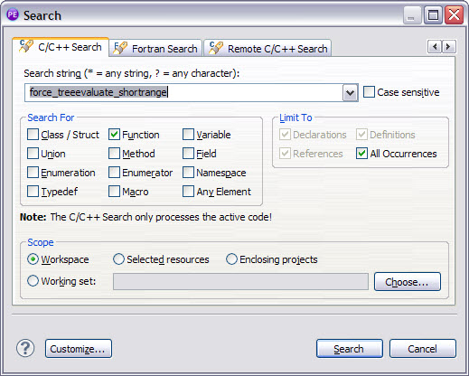
Figure 7-28 Searching for force_treeevaluate_shortrange

Figure 7-29 Opening force_treeevaluate_shortrange implementation
Further information about the Eclipse search in the C/C++ source code is at: Help → Help contents → C/C++ Development User Guide → Tasks → Searching the CDT.
7.3 Analyzing a ScaLAPACK routine using the HPCT Toolkit
ScaLAPACK is a library of high-performance linear algebra routines for parallel distributed memory machines. ScaLAPACK solves dense and banded linear systems, least squares problems, eigenvalue problems, and singular value problems.
In this section, we analyze the performance of the ScaLAPACK routine PDGETRF, which performs an LU factorization of a dense real matrix. This calculation is similar to that used in the well-known Linpack Benchmark.
7.3.1 The Structure of ScaLAPACK
ScaLAPACK is a continuation of the LAPACK project, which contains high-performance linear algebra software for shared memory computers. LAPACK itself is built on top of the well-know Basic Linear Algebra Subprograms (BLAS). The BLAS routines are a set of kernels for performing low-level vector and matrix operation. Since the interfaces to the BLAS routines have been defined to be a de facto standard, computer vendors can provide highly-tuned versions of the BLAS routines, designed to perform optimally on a given architecture.
ScaLAPACK extended the idea of the BLAS and defines a set of BLACS. In this way, high performance can be achieved by confining machine-specific optimizations to the BLAS and BLACS libraries.
The high-level structure of the ScaLAPACK and related library is shown in Figure 7-30.

Figure 7-30 ScaLAPACK structure
The relevant components of the directory structure of the ScaLAPACK distribution are:
SCALAPACK
lapack-3.4.1
BLAS
SRC
scalapack-2.0.2
scalapack-2.0.2
BLACS
PBLAS
SRC
TESTING
LIN
EXAMPLE
The ScaLAPACK library contains an extensive suite of test programs in the scalapack-2.0.2/TESTING directory. Typically these test programs test an individual routine with many different input parameters to test the correctness of the installation. We modified the top-level driver pdludriver.f, used it to build the test program xdlu and to increase the value of the parameter TOTMEM, so that larger problem sizes are handled. We also modified the data file that drives the xdlu program to solve a single large problem, rather than many small ones.
7.3.2 The build process
Both LAPACK and ScaLAPACK have a top-level Makefile, which defines all the build targets and the dependencies. Each of these Makefiles includes a file (make.inc and SLmake.inc, respectively) that defines the compiler options to be used on a particular platform.
Within each directory, we run the following make commands:
lapack-3.4.1
make blaslib
make lapacklib
scalapack-2.0.2
make lib
make scalapackexe
Within the corresponding Eclipse/PTP project, we define these targets by right-clicking the lapack-3.4.1 and scalapack-2.0.2 directories in the Project Explorer window and selecting Make Targets → Build (Alt-F9) → Add.
7.3.3 CPU profiling
The first step in CPU profiling is to perform a CPU hot-spot analysis. To do this, we add the flags -g -pg to lapack-3.4.1/make.inc and scalapack-2.0.2/SLmake.inc, and rebuild the package.
Running the program on a single node:
poe ./xdlu -procs 16
The run generates a series of gmon.out files in the format used by the standard UNIX utility gprof. On the Power architecture, running either Linux or AIX, the Xprof utility can be used to explore these profiles:
source /opt/ibmhpc/ppedev.hpct/env_sh
Xprof ./xdlu prof*/gmon*
The following window appears as shown in Figure 7-31 on page 165.

Figure 7-31 Profile report
We run View → Uncluster functions so that the program call tree is no longer enclosed in the box associated with the program code. This changes the appearance of the window, as shown in Figure 7-32 on page 166.

Figure 7-32 Profile report uncluster view
Next we examine the traditional gprof “flat profile” by selecting Report → Flat Profile (Figure 7-33 on page 167).

Figure 7-33 Flat profile report view
This shows that the overwhelming majority of time, 92.5%, is spent in the Level 3 BLAS routine DGEMM, which is a matrix-matrix multiplication routine. At this point, the obvious course of action is to replace the Fortran BLAS library, distributed with the LAPACK library, with calls to vendor-specific tuned BLAS - ESSL for the IBM Power architecture, or the MKL library for the Intel x86_64 architecture. However, we continue working with the Fortran DGEMM BLAS routine to demonstrate the other tools in the HPCT suite.
It is unusual in real-world applications to find one routine consuming such a high proportion of CPU time, and it is easy to locate the rectangle corresponding to DGEMM in the call graph. Normally, from the flat profile view, we select the line corresponding to DGEMM, and select Tools → Locate in the graph to show the DGEMM rectangle, as shown in Figure 7-34 on page 168.

Figure 7-34 DGEMM rectangle
The rectangle is almost exactly square, showing a large amount of time spent in DGEMM, where all of it is spent in the routine itself and nothing in its children. By right-clicking the DGEMM rectangle and selecting display source code, a window is displayed that shows the source code of the DGEMM routine. Because all of the routines were compiled with the XL compilers’ -qfullpath flag, the tool can locate the source code immediately, without t specifying a path to the source directory.
By scrolling down the window, we find the lines of code where the time is being spent, as shown in Example 7-1.
Example 7-1 Lines of the program where the running time is spent
no. ticks
line per line source code
303 2 DO 90 J = 1,N
304 IF (BETA.EQ.ZERO) THEN
305 DO 50 I = 1,M
306 C(I,J) = ZERO
307 50 CONTINUE
308 ELSE IF (BETA.NE.ONE) THEN
309 DO 60 I = 1,M
310 C(I,J) = BETA*C(I,J)
311 60 CONTINUE
312 END IF
313 18 DO 80 L = 1,K
314 129 IF (B(L,J).NE.ZERO) THEN
315 TEMP = ALPHA*B(L,J)
316 6 DO 70 I = 1,M
317 24093 C(I,J) = C(I,J) + TEMP*A(I,L)
318 70 CONTINUE
319 END IF
320 80 CONTINUE
321 90 CONTINUE
Each tick is a sample of 1/100th second so that 24093 ticks associated with line 317 corresponds to 240.93 seconds of CPU time associated with the line of code.
7.3.4 HPM profiling
The “DO 70” loop in Example 7-1 on page 168 is written so that the arrays are accessed in column major order, which is typically good for Fortran code. However, better performance can usually be achieved by unrolling DO-loops, so that more use is made of each array element that is loaded into cache before that element is discarded.
Such optimizations are typical of the customized BLAS routines available in the IBM ESSL and the Intel MKL libraries. In this case, we use compiler optimizations to show how different levels of optimization can affect the performance of this loop.
In general, hardware performance counters are extremely hard to interpret in absolute terms without detailed knowledge of both the underlying hardware and the application. However, in tuning an application, it is often possible to get some useful information by examining performance counters before and after tuning occurs.
For ScaLAPACK, we instrumented the xdlu executable for gathering HPM information using the command:
hpctInst -dhpm ./xdlu
This command creates the file xdlu.inst. Note that in general it is better to instrument just a few key areas of the code because the full HPM instrumentation adds significantly to the overall run time. We therefore instrumented xdlu using Eclipse/PTP, adding instrumentation ONLY to the call to pdgemm. We choose this, rather than dgemm itself, because this section of code remains unchanged even though next we completely replace the dgemm routine.
First, we run the application using the default HPM Event group. For each task, we obtain a .viz file and a .txt file. First, we examine one of the .txt files and search for the section labelled pdgemm, as shown in Figure 7-35 on page 170.
|
Instrumented section: 1 - Label: pdgemm
process: 3276958, thread: 1
file: pdgemm_.c, lines: 259 <--> 506
Context is process context.
No parent for instrumented section.
Inclusive timings and counter values:
Execution time (wall clock time) : 43.9370487332344 seconds
Initialization time (wall clock time): 0.19987041503191 seconds
Overhead time (wall clock time) : 0.0135871283710003 seconds
PM_FPU_1FLOP (FPU executed one flop instruction) : 17912567
PM_FPU_FMA (FPU executed multiply-add instruction) : 35711748287
PM_FPU_FSQRT_FDIV (FPU executed FSQRT or FDIV instruction) : 0
PM_FPU_FLOP (FPU executed 1FLOP, FMA, FSQRT or FDIV instruction) : 35729660854
PM_RUN_INST_CMPL (Run instructions completed) : 190402795098
PM_RUN_CYC (Run cycles) : 184265923937
Utilization rate : 99.759 %
Instructions per run cycle : 1.033
Total scalar floating point operations : 71441.409 M
Scalar flop rate (flops per WCT) : 1625.995 Mflop/s
Scalar flops per user time : 1629.925 Mflop/s
Algebraic floating point operations : 71441.409 M
Algebraic flop rate (flops per WCT) : 1625.995 Mflop/s
Algebraic flops per user time : 1629.925 Mflop/s
Scalar FMA percentage : 99.975 %
Scalar percentage of peak performance : 9.693 %
|
Figure 7-35 pdgemm output
We note two specific values here: Scalar percentage of peak performance, which is 9.963%, and Algebraic flob rate (flops per WCT), which is 1625.925Mflop/s.
To show the difference, we can potentially tune the dgemm kernel optimally, link the code with the IBM ESSL (Engineering and Scientific Subroutine Library), and repeat the experiment. In this case, we obtain the following information for the pdgemm section, as shown in Figure 7-36 on page 171.
|
Instrumented section: 1 - Label: pdgemm
process: 3670092, thread: 1
file: pdgemm_.c, lines: 259 <--> 506
Context is process context.
No parent for instrumented section.
Inclusive timings and counter values:
Execution time (wall clock time) : 19.9932569861412 seconds
Initialization time (wall clock time): 0.202705550938845 seconds
Overhead time (wall clock time) : 0.0138184614479542 seconds
PM_FPU_1FLOP (FPU executed one flop instruction) : 18123119
PM_FPU_FMA (FPU executed multiply-add instruction) : 35711748287
PM_FPU_FSQRT_FDIV (FPU executed FSQRT or FDIV instruction) : 0
PM_FPU_FLOP (FPU executed 1FLOP, FMA, FSQRT or FDIV instruction) : 35729871406
PM_RUN_INST_CMPL (Run instructions completed) : 61851849877
PM_RUN_CYC (Run cycles) : 83586326217
Utilization rate : 99.446 %
Instructions per run cycle : 0.740
Total scalar floating point operations : 71441.620 M
Scalar flop rate (flops per WCT) : 3573.286 Mflop/s
Scalar flops per user time : 3593.178 Mflop/s
Algebraic floating point operations : 71441.620 M
Algebraic flop rate (flops per WCT) : 3573.286 Mflop/s
Algebraic flops per user time : 3593.178 Mflop/s
Scalar FMA percentage : 99.975 %
Scalar percentage of peak performance : 21.368 %
|
Figure 7-36 pdgemm new output
We now see that the Scalar percentage of peak performance increased to 21.368%, and the Algebraic flop rate (flops per WCT) increased to 3573.286Mflop/s.
The DGEMM routine in ESSL was carefully constructed to make much effective use of the memory hierarchy, so that as much use is made of data loaded into the caches, close to the processor, before calculation needs to be delayed by accessing memory. We can see this by looking at a counter group that lists details of memory access. When we run the Fortran version, and look at group 11, we see the values for the counters shown in Figure 7-37 on page 172.
|
PM_DATA_FROM_MEM_DP (Data loaded from double pump memory) : 0
PM_DATA_FROM_DMEM (Data loaded from distant memory) : 0
PM_DATA_FROM_RMEM (Data loaded from remote memory) : 10345114
PM_DATA_FROM_LMEM (Data loaded from local memory) : 11189436
PM_RUN_INST_CMPL (Run instructions completed) : 191101049438
PM_RUN_CYC (Run cycles) : 185020305804
|
Figure 7-37 Memory counter group details
This can be contrasted with values obtained from the ESSL version of DGEMM, as shown in Figure 7-38.
|
PM_DATA_FROM_MEM_DP (Data loaded from double pump memory) : 0
PM_DATA_FROM_DMEM (Data loaded from distant memory) : 0
PM_DATA_FROM_RMEM (Data loaded from remote memory) : 2878806
PM_DATA_FROM_LMEM (Data loaded from local memory) : 2243331
PM_RUN_INST_CMPL (Run instructions completed) : 62033373737
PM_RUN_CYC (Run cycles) : 83109304433
|
Figure 7-38 Values from the ESSL version of DGEMM
We can see clearly from these statistics that the ESSL DGEMM routine loads far less data from memory.
Raw performance counters can also be examined using the peekperf GUI, as shown in Figure 7-39 on page 173.

Figure 7-39 Raw performance counters shown using the peekperf GUI
7.3.5 MPI profiling
We next perform MPI profiling, which can be enabled by linking with the libmpitrace library. We access the PEDE environment variables source /opt/ibmhpc/ppedev.hpct/env_sh and add the following syntax to the link step in the file TESTING/LIN/Makefile:
-L$(IHPCT_BASE)/lib64 -lmpitrace
Alternatively, we can use dynamic instrumentation to add tracing to a prebuilt executable:
hpcInst -dmpi xdlu
Although we do not modify the source code to alter the communications patterns, we can still influence the way the code performs by modifying some of the parameters in the input file.
One of the key parameters that affects the performance of ScaLAPACK routines is the block size, given by MB in the input file. If the block size in linear algebra routines is too small, excessive amounts of communication with small messages is generated. On the other hand, if the block size is too large, the blocks will be too large to fit into the processor cache, so that the reduction in communications is offset by the reduced computational efficiency.
To illustrate this, we show the textual MPI profile information and the graphical display of MPI calls for the two cases where NB=32 (which is a reasonably good value for the Fortran code), and NB=256 (which is too large). In each case, we request that information be collected for all tasks, and all events are also collected to the trace file. To achieve this, we set the following environment variables:
export OUTPUT_ALL_RANKS=yes
export TRACE_ALL_TASKS=yes
export TRACE_ALL_EVENTS=yes
We found initially that the default number of events to trace, 30,000, was too small, and se we increased it as follows:
export MAX_TRACE_EVENTS=500000
Examining the file hpct_0_0.mpi.txt, the trace from task 0, for NB=32 is shown in Figure 7-40.
|
-----------------------------------------------------------------
MPI Routine #calls avg. bytes time(sec)
-----------------------------------------------------------------
MPI_Comm_size 1 0.0 0.0000
MPI_Comm_rank 3 0.0 0.0000
MPI_Send 3428 32055.3 0.101
MPI_Rsend 6 8.0 0.0000
MPI_Isend 47755 2307.9 0.249
MPI_Recv 56648 3861.0 6.608
MPI_Testall 47755 0.0 0.048
MPI_Waitall 473 0.0 0.000
MPI_Bcast 9341 15476.4 1.248
MPI_Barrier 2 0.0 0.020
MPI_Reduce 789 1270.8 0.207
MPI_Allreduce 37 5.9 0.004
-----------------------------------------------------------------
total communication time = 8.485 seconds.
total elapsed time = 56.336 seconds.
|
Figure 7-40 hpct_0_0.mpi.txt output file
The bottom of this file is shown in Figure 7-41.
|
Communication summary for all tasks:
minimum communication time = 8.485 sec for task 0
median communication time = 9.411 sec for task 4
maximum communication time = 10.226 sec for task 14
|
Figure 7-41 hpct_0_0.mpi.txt bottom section
The corresponding sections of the task 0 trace file when NB=256 are shown in Figure 7-42 on page 175.
|
-----------------------------------------------------------------
MPI Routine #calls avg. bytes time(sec)
-----------------------------------------------------------------
MPI_Comm_size 1 0.0 0.0000
MPI_Comm_rank 3 0.0 0.000
MPI_Send 515 411610.2 0.442
MPI_Rsend 6 8.0 0.000
MPI_Isend 45691 2367.4 0.223
MPI_Recv 52190 6067.0 16.339
MPI_Testall 45691 0.0 0.046
MPI_Waitall 128 0.0 0.000
MPI_Bcast 6555 626.8 0.126
MPI_Barrier 2 0.0 0.031
MPI_Reduce 237 4286.7 0.860
MPI_Allreduce 37 5.9 0.002
-----------------------------------------------------------------
total communication time = 18.069 seconds.
total elapsed time = 97.995 seconds.
|
Figure 7-42 Task 0, NB = 256
The communication summary of all tasks is shown in Figure 7-43.
|
Communication summary for all tasks:
minimum communication time = 14.504 sec for task 9
median communication time = 18.069 sec for task 0
maximum communication time = 24.945 sec for task 15
|
Figure 7-43 Communication summary
A summary of MPI communications can be obtained by loading the .viz files into the peekperf GUI, as shown in Figure 7-44 on page 176.

Figure 7-44 .viz file into the peekperf GUI
It is also instructive to examine the communications patterns for both cases. We examine the .mpt file using the peekview GUI. In both cases, we present two views: the first is zoomed in to show approximately one second of execution, and the second zooms in further to show approximately 0.2 seconds.
For the NB=32 example, the second view is shown in Figure 7-45 on page 177.

Figure 7-45 NB case second view
For the NB=32 case, the 0.2 second view is shown in Figure 7-46.

Figure 7-46 NB=32 case 0.2 view
For the NB=256 case, the one second view is shown in Figure 7-47 on page 178.

Figure 7-47 Communication phase
We see that the communications phase lasts nearly the full second in this case. The 0.2 second view, zooming in on the busy part, is shown in Figure 7-47.
Figure 7-48 shows the peekperf trace view.
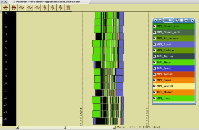
Figure 7-48 Peekperf trace view
..................Content has been hidden....................
You can't read the all page of ebook, please click here login for view all page.