


Parallel Environment Developer Edition tools
This chapter describes the use of the IBM Parallel Environment (PE) Developer Edition tools that are available to assist you with several kinds of performance analysis, tuning, debugging, and for solving issues in parallel applications.
These tools are mostly integrated within the Eclipse IDE, designed to be easily executed and still grant flexibility. They provide assistance in finding hot spots in source code, performance bottlenecks, and also are helpful in finding malfunctions and defects in parallel applications.
This chapter provides information about:
6.1 Tuning tools
The IBM HPC Toolkit provides profiling and trace tools integrated within the Eclipse UI and that are designed to gather rich data regarding the parallel application behavior in execution time. Therefore, it is recommended to use these tools to obtain initial performance measurements for your application, find hotspots, and also bottlenecks.The tools are:
•HPM tool for performance analysis based on hardware event counters
•MPI profiling and trace tool for performance analysis based on MPI events
•OpenMP profiling and trace tool for performance analysis of openMP primitives
•I/O profiling tool for performance analysis of parallel application I/O activities
There is the non eclipse-integrated Xprof tool, which is distributed within PEDE and relies on call graph base analysis for performance analysis. Its use is actually recommended first in the tuning process because it gets an overview of performance problems and is also suitable for identifying functions wasting most of the application execution time.
Our suggestion is to start identifying hotspots with Xprof and then narrow down the problem using other tools.
The basic workflow to use the Eclipse-integrated tools is illustrated in Figure 6-1 on page 97, where you start by preparing the application for profiling. After that, you must make a profile launch configuration according to your needs and then you must run the application to obtain data. Finally you get to visualize results in many possible ways with information presented at several levels of detail allowing operations, such as zooming in/out and easy browsing through the data collected.

Figure 6-1 IBM HPC Toolkit basic workflow
All data is produced and collected in application runtime through the use of some technologies that require your application’s executable be instrumented. Indeed, the IBM HPC Toolkit instrumentation mechanism enables you to focus on just a small portion of code to avoid common problems on application analysis, for instance, increased overhead and production of uninteresting data. The instrumentation mechanisms are explained in 6.1.1, “Preparing the application for profiling” on page 100.
An overview about how to create a profile launch configuration is shown in 6.1.2, “Creating a profile launch configuration” on page 104. This is an essential step in the workflow where you configure a tool for execution and the IBM HPC Toolkit allows you to determine the detail level and amount of performance data to be collected.
The tools support varies based on the target environment (operating system and hardware architecture) where an application is built to run in. Table 6-1 presents the tools support by environments.
Table 6-1 Tools supported by platform
|
Tool
|
Linux on x86
|
Linux on Power1
|
AIX on IBM Powera
|
|
Xprof
|
No
|
Yes
|
Yes
|
|
Hardware Performance Monitor
|
Yes 2
|
Yes
|
Yes
|
|
I/O Profiler
|
Yes
|
Yes
|
Yes
|
|
MPI Profiler
|
Yes
|
Yes
|
Yes
|
|
OpenMP Profiler
|
No
|
Yes
|
Yes
|
1 Currently supports IBM POWER6 and POWER7 processors and application built with the IBM XL Compiler only.
2 Currently supports Intel x86 Nehalem, Sandy Bridge, and Westmere microarchitectures.
The IBM HPC Toolkit Eclipse perspective
The IBM HPC Toolkit plug-in comes with an eclipse perspective (“Eclipse terms and concepts” on page 5) that consolidates tooling operations conveniently into a single view to support the following tasks:
•Instrument binaries in preparation to run analysis
•Manage, browse and one-click visualize performance data
•Configure visualization modes
•The bottom-left Instrumentation view allows binary instrumentation for ease. It contains tabs to instrument your binaries by selecting options specific for each tools. It also holds a button to trigger instrumentation. More information about binary instrumentation is provided in “Preparing the application for profiling” on page 100.
•The bottom-right Performance Data tab view lists all generated performance data files of your project. It also allows you to browse data generated by different tools and a double-click in any file name is going to open its associated visualization into the Performance Data Summary tab view.
The bottom-right Performance Data Summary tab view is where the gathered data actually showed up in table report format.
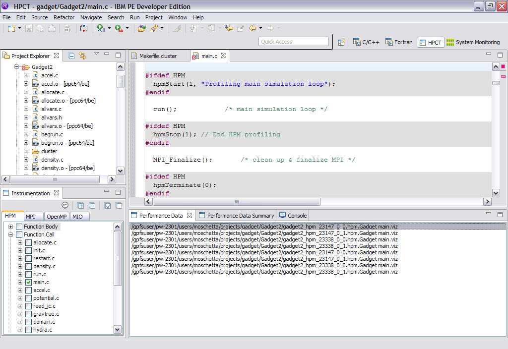
Figure 6-2 IBM HPC Toolkit Eclipse perspective
There are other views specific to some tools because of the different visualization required and so will appear eventually. They will be detailed later in this chapter, thus following are just their names for reference:
•Metric browser
•MIO detail
•MIO summary
•MIO trace
•MPI trace
•Performance data detail
The perspective can be opened in several ways, for instance:
•On top menu bar, click Window → Open perspective → Other. Select HPCT from the Open perspective window and then click OK.

Figure 6-3 Open perspective button

Figure 6-4 Open perspective window
6.1.1 Preparing the application for profiling
There are two requirements a parallel application must match to be analyzed by IBM HPC Toolkit tools:
•The parallel application executable must be instrumented by changing either its source code or binary file so that the IBM HPC Toolkit can get performance data.
•The parallel application must be built with the -g flag. Also, if chose binary instrumentation in a Linux on IBM Power system then it requires also -Wl,--hash-style=sysv -emit-stub-syms flags, as shown in the excerpt of Makefile in Example 6-1.
Example 6-1 Using the IBM HPC Toolkit required build flags in the Makefile
# HPC Toolkit required flags
HPCT_OPTS = -g -Wl,--hash-style=sysv -emit-stub-syms
LIBS = $(HDF5LIB) -g $(MPICHLIB) $(GSL_LIBS) -lgsl -lgslcblas -lm $(FFTW_LIB)
$(EXEC): $(OBJS)
$(CC) $(OBJS) $(LIBS) $(HPCT_OPTS) -o $(EXEC)
$(OBJS): $(INCL)
clean:
rm -f $(OBJS) $(EXEC)
Instrumenting the application
The toolkit is flexible enough to allow you to instrument a whole program, but also just the smallest areas of it where you might be interested in analyzing performance with the advantages of giving you control over the areas of your application that you want to analyze (zoom in/out) and, consequently, the amount of data gathered.
The toolkit provides you with two modes1 of instrumentation:
•Code instrumentation: Application code must be rewritten and recompiled with calls to the toolkit instrumentation library.
•Binary instrumentation2 3: Application executable is rewritten by the toolkit with the instrumentation specified by you.
Code instrumentation
In the code instrumentation model, you must insert certain API calls into your application code so that you specify start/stop of profiling and regions performance data that must be collected. The IBM HPC Toolkit provides different runtime libraries, API, and linkage procedures for each of the performance tools (Table 6-2) so more details about the usage of code instrumentation is given in the tools section.
Table 6-2 IBM HPC Toolkit runtime libraries and headers
|
Library
|
Description
|
C header1
|
Fortran headera
|
|
hpc
pmapi2
|
Provides instrumentation and analysis for Hardware Performance Monitoring tool
|
libhpc.h
|
f_hpc.h
f_hpc_i8.h
|
|
mpitrace
|
Provides analysis for the MPI Profile and Trace tool
|
mpt.h
|
mpt_f.h
|
|
hpctkio
|
Provides analysis for the IO Profile tool
|
hpcMIO_user.h
|
Not supported
|
1 Header files are located in /opt/ibmhpc/ppedev.hpct/include
2 Only for AIX Systems
Binary instrumentation
In the binary instrumentation model, you use an GUI tool to select regions of your application that will be instrumented. The instrumentation tool is in charge of providing you the options as well as rewrite the application executable within all needed instructions to gather data for an specific HPCT. Notice that such as modality of instrumentation is straightforward in most of the cases but as stated before it isn’t supported in x86 Linux systems that in turn will require source code change.
Binary instrumentation can be accomplished in three steps:
1. Open the executable for instrumentation. Within the project opened in the Project Explorer view, right-click the binary and then select HPCT → Open executable (Figure 6-5 on page 102). The HPC Toolkit (HPCT) perspective is automatically opened (refer to “The IBM HPC Toolkit Eclipse perspective” on page 98).
2. Select one or more regions that you are interested in investigating performance and so must be instrumented. Figure 6-6 on page 103 shows an example of binary instrumentation in preparation to run the HPM tool.
3. Click Instrument to generate an instrumented version of the binary with filename <executable>.inst, as shown in Figure 6-7 on page 103.

Figure 6-5 Opening executable for binary instrumentation

Figure 6-6 IBM HPC Toolkit perspective with Instrumentation view
In Figure 6-6, the bottom-left Instrument view has tabs for the tuning tools because each one allows different portions of the binary to be instrumented. So you must change the tab and choose options based on the tool that you want to generate an instrumented executable for analysis. In general, for the tools to work correctly, you must instrument at least one function or an entire source file of the parallel application to obtain performance measurements.
|
Important: Do not mix different tools in a single instrumentation because they might interfere with each other’s analysis in an unpredictable way.
|
After you select the set of instrumentation that you want, you trigger the instrumentation tool by either pressing the instrumentation button in the view or right-clicking the selected node. Click Instrument Executable, as shown in Figure 6-7.

Figure 6-7 Running binary instrumentation tool
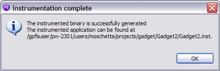
Figure 6-8 Message displayed when instrumentation complete
6.1.2 Creating a profile launch configuration
The IBM HPC Toolkit provides profiling and tracing tools that are useful for performance analysis as long as you properly create a profile launch configuration according to the tool that you want to use and the information you want to observe.
The IBM HPC Toolkit tools are executed by creating and invoking a profile configuration, where that profile configuration is created as a parallel application profile configuration, accessible by right-clicking the project folder and then selecting Profile As → Profile Configurations. It is going to open the Profile Configurations window where new profile launcher configurations are created under the parallel application section in the left box (Figure 6-9).

Figure 6-9 Profile configurations window
The parallel application configuration has Resources, Application, Arguments, and Environments tabs that must be fulfilled with information about how to run the parallel application. In particular, in the Application tab, it must be selected to run the instrumented executable (file named <executable>.inst by default) as illustrated in Figure 6-10.

Figure 6-10 Profile configuration: set instrumented binary
There is also the HPC Toolkit tab that is omitted in Figure 6-10, but it is important to be properly filled because it is actually where you choose what performance tool is executed as well as placing information about how to control data gathering. Figure 6-11 illustrates how to open the HPC Toolkit tab.

Figure 6-11 Opening HPC Toolkit tab
Data collection Contains fields which information is common for the tools.
HPM Contains specific fields to control the HPM tool (Refer to the “Hardware Performance Monitoring” on page 107).
MPI Contains specific fields to control the MPI tracing tool (Refer to the “MPI profiling and trace” on page 111).

Figure 6-12 HPC Toolkit tab
The data collection tab (see Figure 6-12) is where you control the amount of data gathered in the process. Their fields must be carefully fulfilled, especially on large task applications where you really must limit the number of tasks that the tool generates data from, both to avoid file system performance impacts of generating thousands of files worth of data and from the impracticality of you managing and analyzing all of that data. The following list contains an explanation of each field:
•The Output File Name field value defines the base name for performance files generated by the tool, and the name will be <basename>_<world_id>_<world_rank>. Set it with a meaningful value for the particular tool you intend to run.
•The Generate Unique File names check box ensures that performance data files are separately generated by each MPI task. You must enable it if running an MPI application.
•The hpcrun check box allows you to change data collection behavior. If not enabled, the tool gets data for all tasks, except as limited by environment variables described for MPI profiling and the trace tool (refer to “MPI profiling and trace” on page 111). If enabled, you must set its nested fields:
– Application time criteria specifies the metric the tool uses to decide what tasks to collect data from, either wall clock (ELAPSED_TIME) or CPU time (CPU_TIME).
– Exception task count field limits the number of tasks the tool generates data from. You must specify the minimum and maximum number of data tasks that will be collected along with the average task and task 0.
– Trace collection mode specifies how the tool uses system memory to collect data. There are two values accepted:
• Memory is appropriate for applications generating small trace files which do not steal memory from the application's data space
• Intermediate is appropriated for applications generating larger trace files
6.1.3 Hardware Performance Monitoring
The Hardware Performance Monitoring (HPM) tool leverages the hardware performance counters for performing low level analysis, which are quite helpful to identify and eliminate performance bottlenecks.
HPM allows you to obtain measurements on:
•Single hardware counter group of events
•Multiple hardware counter group of events
•Pre-defined metrics based on hardware counter group of events. Examples of derived metrics are:
– Instructions per cycles
– Branches mispredicted percentage
– Percentage of load operations from L2 per cycle
Profiling your application
To profile your application:
1. Build the application using the required flags, as described in “Preparing the application for profiling” on page 100.
2. Instrument the parallel application in one of the following modes (see“Instrumenting the application” on page 100 for the basics on instrumentation):
a. Instrument source code by calling HPM runtime library functions. The application must be recompiled with some flags according to the run environment, as shown in Table 6-3. Refer to Table 6-4 for a quick reference to the runtime library API or consult the IBM HPC Toolkit manual at:
Table 6-3 Build settings quick reference
|
|
Compiler options
|
Linker options
|
Headers
|
|
Linux
|
-g
-I/opt/ibmhpc/ppedev.hpct/include
|
-lhpc
-L/opt/ibmhpc/ppedev.hpct/lib or -L/opt/ibmhpc/ppedev.hpct/lib64
|
libhpc.h
|
|
AIX
|
-g
-I/opt/ibmhpc/ppedev.hpct/include
|
-lhpc
-lpmapi
-lpthreads3
-L/opt/ibmhpc/ppedev.hpct/lib or
-L/opt/ibmhpc/ppedev.hpct/lib64
|
libhpc.h
f_hpc.ha or f_hpc_i8.hb
|
1 Fortran applications
2 Fortran applications compiled with -qintsize=8
3 Optionally use xlc_r or xlf_r with IBM XL C/C++/Fortran compiler
Table 6-4 HPM library API quick reference
|
Description
|
C/C++
|
Fortran
|
|
Initialize the instrumentation library
|
hpmInit(id, progName)
|
f_hpminit(id, progName)
|
|
Terminate the instrumentation library and generate the reports
|
hpmTerminate(id)
|
f_hpmterminate(id)
|
|
Identify the start of a section of code in which hardware performance counter events are counted
|
hpmStart(id, label)
|
f_hpmstart(id, label)
|
|
Identify the end of the section of code in which hardware performance counter events were counted
|
hpmStop(id)
|
f_hpmstop(id)
|
b. Instrument executable by leveraging the instrumentation tool that is going to produce a new binary renamed <executableName>.inst. Figure 6-13 shows the instrumentation tool allowing you to select any combination of three classes of instrumentation:
• Function call sites
• Entry and exit points of function
• User-defined region of code

Figure 6-13 Instrumenting a binary for HPM profiling
3. Create an HPM launcher configuration where you must fulfill fields to control the data produced and gathered (refer to “Creating a profile launch configuration” on page 104). Figure 6-14 on page 109 shows the tool configuration screen that requires input of either a derived metric or counter group number.
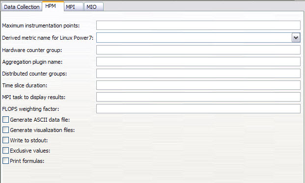
Figure 6-14 HPM configuration screen
The tool comes with existing derived metrics that are in most of the cases a good starting point for hardware performance analysis because they will result in higher-level information than just raw hardware events data. However, it still allows you to gradually pick events that show more hardware information in more low level hardware toward a performance bottleneck. Figure 6-15 lists every pre-built hardware performance metrics of Linux on IBM POWER7.

Figure 6-15 Derived hardware performance metrics for Linux on POWER7
However, you might want to use one of many counter groups available in your processor instead of the derived metrics. The listing of the counter groups must be obtained by manually connecting at the target system and executing the hpccount command, as shown in Example 6-2. Run man hpccount to open its manual and thus check out other useful options.
Example 6-2 Listing hardware performance groups
$ source /opt/ibmhpc/ppedev.hpct/env_sh
$ hpccount -l | less
Figure 6-16 shows the output of Example 6-2 executed in a POWER7 machine. Notice that the report shows the total of counter groups for the given processor and the complete listing of groups along with their associated hardware events.

Figure 6-16 Example: output of command hpccount -l
Interpreting profile information
The HPCT perspective is opened as soon as profiling finishes. After which you are prompted to open the visualization files.
Figure 6-17 on page 111 shows an example of HPM results visualization for an application, which main.c function was instrumented (see bottom-left Instrumentation view). The tool collected hardware counter data, formatted it, and then wrote in visualization files (see listing in bottom-right Performance Data view).
All generated information regarding hardware performance data is displayed in the Performance Data Summary view, as shown in Figure 6-22 on page 114.
Figure 6-17 HPM performance data list
6.1.4 MPI profiling and trace
The MPI profiling and trace tool from IBM HPC Toolkit can gather data for all MPI routines and then generate profile reports and trace visualization of MPI primitives. However, currently the tool cannot create a trace for an application that issues MPI function calls from multiple threads in the application.
Instrumenting your application
To instrument your application, refer to the following steps:
1. To perform the profiling, either the binary can be instrumented by opening the binary directly using Eclipse or linking the source code with the libmpitrace.so for Linux and libmpitrace.a for AIX and then recompiling it. The application must be built using the required flags, as described in “Preparing the application for profiling” on page 100.
Currently the binary instrumenting without re-compilation approach is only supported on the POWER based architecture.
Figure 6-18 on page 112 illustrates how to link your source code to perform MPI profiling on a x86-based Linux machine. The source code mpi_1.c is utilized in this example as a Makefile project. Simply link the libmpitrace into your makefile.

Figure 6-18 Linking the libmpitrace
The mpi_1.c is linked to the mpitrace lib:
-L/opt/ibmhpc/ppedev.hpct/lib64 -lmpitrace
Notice that the linking is added to the end of this line; otherwise, the mpi tracing data might not be generated properly. Having done so, you might want to configure the profiling by clicking Profile and then choosing the profile configuration. On the left of the pop-up window, click Parallel Application to create a new profile configuration, as shown in Figure 6-19.

Figure 6-19 Creating a new profile configuration
In the resource tab, choose IBM Parallel Environment for the Target System configuration. Click the HPC Toolkit tab and populate the name for the profiling data files, as shown in Figure 6-20 on page 113.

Figure 6-20 Adding the name for the profile data file
You can leave others as default. By default, the MPI profiling library will generate trace files only for the application tasks with the minimum, maximum, and median MPI communication time. This is also true for task zero, if task zero is not the task with minimum, maximum, or median MPI communication time. If you need trace files generated for additional tasks, make sure Output trace for all tasks or the OUTPUT_ALL_RANKS environment variable is set correctly. Depending on the number of tasks in your application, make sure Maximum trace rank and Limit trace rank or MAX_TRACE_RANK and TRACE_ALL_TASKS environment variables are set correctly. If your application executes many MPI function calls, you might need to set the value of Maximum trace events or the MAX_TRACE_EVENTS environment variable to a higher number than the default 30,000 MPI function calls. Click Profile on the bottom of the pop-up window. After the program completes, some profiling data is generated in your working directory (see .viz files in Figure 6-21 as an example) that is read in automatically by Eclipse.
Figure 6-21 Profiling data generation
The performance data then is shown as a readable format in the HPCT perspective window, as shown in Figure 6-22 on page 114. Each of the MPI routines is tracked, which presents the consumed time and the amount of invoking times. Hence it is easy to analyze the communication overhead of MPI in a parallel application with this data.

Figure 6-22 Performance data summary
In addition, the raw data can be presented in a more visual way, as shown in Figure 6-23 on page 115. The Y axis is the application task rank, and the X. If you put the cursor on it in PEDE, more detailed information is displayed.
To open the MPI trace view:
1. Right-click in the performance data summary, and click the load trace option in the pop-up menu.
2. Select a path to store a local copy of the trace file in the pop-up file selector dialog. Click OK → Open. In the MPI Trace window, click Load Trace.
3. Choose the corresponding file with the extension name .mpt for loading.

Figure 6-23 Data representation pictorially
6.1.5 OpenMP profiling
Binary instrumenting is the only way to profile OpenMP, and the application must be compiled with -g -Wl,--hash-style=sysv -emit-stub-syms compiler flags on a Linux on POWER based system (x86 architecture is not currently supported) or with -g for AIX. Besides, the IBM HPC Toolkit only supports OpenMP profiling instrumentation for OpenMP regions that are not nested within other OpenMP constructs at run time. If you set up instrumentation so that nested parallel constructs are instrumented, the results are unpredictable:
1. After the application is properly compiled, right-click the executable from the Eclipse project window, and choose the HPCT → Open executable, as shown in Figure 6-24 on page 116.
2. Choose what you want to instrument from the OpenMP tab in the Instrumentation view.
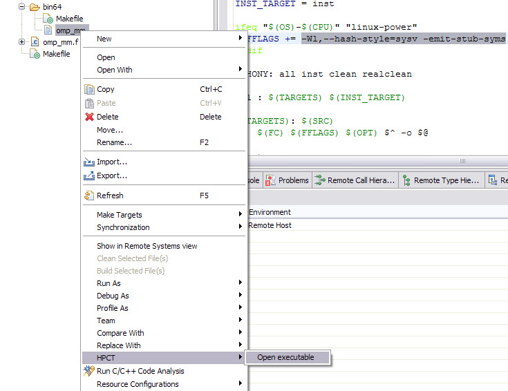
Figure 6-24 Open a executable file for instrumentation
3. Right-click what you chose, and perform the instrumentation, as shown in Figure 6-25. A instrumented executable is created with the .inst extension name.

Figure 6-25 Choose openmp source code to instrument
1. Some profiling raw data is generated by running the instrumented binary. After synchronizing from the remote machine, try to open the .viz files using Eclipse. You will see profiling data, as shown in Figure 6-26 on page 117.
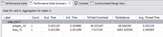
Figure 6-26 Sample OpenMP profiling result
6.1.6 I/O profiling
I/O profiling is where you can obtain information about I/O calls made in your application to help you understand application I/O performance and identify possible I/O performance problems in your application. For example, when an application exhibits the I/O pattern of sequential reading of large files, when environment variables are set appropriately, MIO detects the behavior and invokes its asynchronous prefetching module to prefetch user data.
Currently the MIO tool is only available for parallel applications written in C language and also only able to collect data regarding system I/O library calls (not standard I/O).
Preparing your application
Your application must be compiled and linked with the –g compiler flag. When you compile an application on a Power Linux system, you must also use the -Wl,--hash-style=sysv -emit-stub-syms compiler flags. For example, there is a sample included in the HPCT package located in the /opt/ibmhpc/ppedev.hpct/examples/mio directory. The original Makefile under the bin64 and the bin32 subdirectory is already linked with the HPCT library. However we need to do some modifications, as shown in Example 6-3.
Example 6-3 Modification for Makefile in bin64 subdirectory
TARGETS = fbs
OBJS = fbs.o FBS_encode_data.o FBS_str_to_long.o rtc.o
#LDFLAGS += -L$(IHPCT_BASE)/lib64 -lhpctkio
LDFLAGS += -Wl,--hash-style=sysv -emit-stub-syms
To prepare your application:
1. Create a new project named mio, and synchronize the project with the remote host.

Figure 6-27 Open the project mio
3. Perform the Make Targets → Build to generate executable binary fbs.
Instrumenting your application
To instrument your application:
1. Select fbs and right-click it. Select HPCT → Open executable, in the Instrumentation Tab we can see images as shown in Figure 6-28 on page 119.

Figure 6-28 HPCT → Open executable
The MIO view shows the application structure tree fully expanded. The leaf nodes are labeled with the name of the system call at the location and the line number in the source file. If you select leaf nodes, instrumentation is placed only at these specific instrumentation points. If you select a non-leaf node, instrumentation is placed at all leaf nodes that are child nodes of the selected non-leaf node.
For I/O profiling to work correctly, you must instrument at least the open and close system calls that open and close any file for which you want to obtain performance measurements.
2. After you select the set of instrumentation that you want, instrument the application by right-clicking the selected node.

Figure 6-29 Instrument executable

Figure 6-30 The instrumented binary is successfully generated
Instrumenting your application manually
Sometimes we must instrument manually. You must ensure that several environment variables required by the IBM HPC Toolkit are properly set before you use the I/O profiling library. Run the set up scripts located in the top-level directory of your installation, which is normally in the /opt/ibmhpc/ppedev.hpct directory. If you use sh, bash, ksh or a similar shell command, invoke the env_sh script as .env_sh. If you use csh, invoke the env_csh script as source env_csh.
To profile your application, you must link your application with the libhpctkio library using the -L$IHPCT_BASE/lib and -lhpctkio linking options for 32-bit applications or using the -L$IHPCT_BASE/lib64 and -lhpctkio linking options for 64-bit applications.
You must also set the TKIO_ALTLIB environment variable to the path name of an interface module used by the I/O profiling library before you invoke your application:
•For 32-bit applications, set the TKIO_ALTLIB environment variable to $IHPCT_BASE/lib/get_hpcmio_ptrs.so.
•For 64-bit applications, set the TKIO_ALTLIB environment variable to $IHPCT_BASE/lib64/get_hpcmio_ptrs.so.
Optionally, the I/O profiling library can print messages when the interface module is loaded, and it can abort your application if the interface module cannot be loaded.
For the I/O profiling library to display a message when the interface module is loaded, you must append /print to the setting of the TKIO_ALTLIB environment variable. For the I/O profiling library to abort your application if the interface module cannot be loaded, you must append /abort to the setting of the TKIO_ALTLIB environment variable. You might specify one, both, or non of these options.
Note that there are no spaces between the interface library path name and the options. For example, load the interface library for a 64-bit application, display a message when the interface library is loaded, and abort the application if the interface library cannot be loaded. Issue the following command:
export TKIO_ALTLIB=”$IHPCT_BASE/lib64/get_hpcmio_ptrs.so/print/abort”
During the run of the application, the following message prints:
TKIO : fbs : successful load("/opt/ibmhpc/ppedev.hpct//lib64/get_hpcmio_ptrs.so") version=3013
Environment variables for I/O profiling
I/O profiling works by intercepting I/O system calls for any files that you want to obtain performance measurements. To obtain the performance measurement data, the IBM HPC Toolkit uses the I/O profiling options (MIO_FILES) settings and other environment variables.
The first environment variable is MIO_FILES, which specifies one or more sets of file names and the profiling library options to be applied to that file, where the file name might be a pattern or an actual path name.
The second environment variable is MIO_DEFAULTS, which specifies the I/O profiling options to be applied to any file whose file name does not match any of the file name patterns specified in the MIO_FILES environment variable. If MIO_DEFAULTS is not set, no default actions are performed.
The file name that is specified in the MIO_FILES variable setting might be a simple file name specification, which is used as-is, or it might contain wildcard characters, where the allowed wildcard characters are:
•A single asterisk (*), which matches zero or more characters of a file name.
•A question mark (?), which matches a single character in a file name.
•Two asterisks (**), which match all remaining characters of a file name.
The I/O profiling library contains a set of modules that can be used to profile your application and to tune I/O performance. Each module is associated with a set of options. Options for a module are specified in a list and are delimited by / characters. If an option requires a string argument, that argument must be enclosed in brackets {}, if the argument string contains a / character.
Multiple modules can be specified in the settings for both MIO_DEFAULTS and MIO_FILES. For MIO_FILES, module specifications are delimited by a pipe (|) character. For MIO_DEFAULTS, module specifications are delimited by commas (,).
Multiple file names and file name patterns can be associated with a set of module specifications in the MIO_FILES environment variable. Individual file names and file name patterns are delimited by colon (:) characters. Module specifications associated with a set of file names and file name patterns follow the set of file names and file name patterns and are enclosed in square brackets ([]).
The run.sh script under bin64 subdirectory, already include MIO_DEFAULTS and MIO_FILES environment variable settings.
As an example of the MIO_DEFAULTS environment variable setting, assume that the default options for any file that does not match the file names or patterns specified in the MIO_FILES environment variable are that the trace module is to be used with the stats, mbytes, and inter options, and the pf module is to be used with the stats option.
export MIO_DEFAULTS="trace/mbytes/stats/inter,pf/stats"
As an example of using the MIO_FILES environment variable, assume that the application does I/O to *.dat. The following setting will cause files matching *.dat to use the trace module with global cache, stats, xml, and events options.
export MIO_FILES="*.dat[trace/global=pre_pf/stats={stats}/xml/events={evt} ]"
You can just include those environment variable settings in run.sh or put them in the MIO sub-tab under the HPC Toolkit tab in Profile Configurations, as shown in Figure 6-31.

Figure 6-31 MIO sub-tab under HPC Toolkit tab
MIO_DEFAULTS refer to Default profiling options, and MIO_FILES refer to I/O profiling options.
Specifying I/O profiling library module options
Table 6-5 MIO analysis modules
|
Module
|
Purpose
|
|
mio
|
The interface to the user program
|
|
pf
|
A data prefetching module
|
|
trace
|
A statistics gathering module
|
|
recov
|
Analyzes failed I/O accesses and retries in case of failure
|
Table 6-6 MIO module options
|
Option
|
Purpose
|
|
mode=
|
Override the file access mode in the open system call.
|
|
nomode
|
Do not override the file access mode.
|
|
direct
|
Set the O_DIRECT bit in the open system call.
|
|
nodirect
|
Clear the O_DIRECT bit in the open system call.
|
The default option for the mio module is nomode. The pf module has the options, as shown in Table 6-7.
Table 6-7 MIO pf module options
|
Option
|
Purpose
|
|
norelease
|
Do not free the global cache pages when the global cache file usage count goes to zero.
The release and norelease options control what happens to a global cache when the file usage count goes to zero. The default behavior is to close and release the global cache. If a global cache is opened and closed multiple times, there can be memory fragmentation issues at some point. Using the norelease option keeps the global cache opened and available, even if the file usage count goes to zero.
|
|
release
|
Free the global cache pages when the global cache file usage count goes to zero.
|
|
private
|
Use a private cache. Only the file that opens the cache might use it.
|
|
global=
|
Use global cache, where the number of global caches is specified as a value between 0 and 255. The default is 1, which means that one global cache is used.
|
|
asynchronous
|
Use asynchronous calls to the child module.
|
|
synchronous
|
Use synchronous calls to the child module.
|
|
noasynchronous
|
Alias for synchronous.
|
|
direct
|
Use direct I/O.
|
|
nodirect
|
Do not use direct I/O.
|
|
bytes
|
Stats output is reported in units of bytes.
|
|
kbytes
|
Stats is reported in output in units of kbytes.
|
|
mbytes
|
Stats is reported in output in units of mbytes.
|
|
gbytes
|
Stats is reported in output in units of gbytes.
|
|
tbytes
|
Stats is reported in output in units of tbytes.
|
|
cache_size=
|
The total size of the cache (in bytes), between the values of 0 and 1GB, with a default value of 64 K.
|
|
page_size=
|
The size of each cache page (in bytes), between the value of 4096 bytes and 1 GB, with a default value of 4096.
|
|
prefetch=
|
The number of pages to prefetch, between 1 and 100, with a default of 1.
|
|
stride=
|
Stride factor, in pages, between 1 and 1G pages, with a default value of 1.
|
|
stats=
|
Output prefetch usage statistics to the specified file. If the file name is specified as mioout, or no file name is specified, the statistics file name is determined by the setting of the MIO_STATS environment variable.
|
|
nostats
|
Do not output prefetch usage statistics.
|
|
inter
|
Output intermediate prefetch usage statistics on kill -USR1.
|
|
nointer
|
Do not output intermediate prefetch usage statistics.
|
|
retain
|
Retain file data after close for subsequent reopen.
|
|
noretain
|
Do not retain file data after close for subsequent reopen.
|
|
listio
|
Use listio mechanism.
|
|
nolistio
|
Do not use listio mechanism.
|
|
tag=
|
String to prefix stats flow.
|
|
notag
|
Do not use prefix stats flow.
|
The default options for the pf module are:
/nodirect/stats=mioout/bytes/cache_size=64k/page_size=4k/ prefetch=1/asynchronous/global/release/stride=1/nolistio/notag
Table 6-8 MIO trace module options
|
Option
|
Purpose
|
|
stats=
|
Output trace statistics to the specified file name. If the file name is specified as mioout, or no file name is specified, the statistics file name is determined by the setting of the MIO_STATS environment variable.
|
|
nostats
|
Do not output statistics on close.
|
|
events=
|
Generate a binary events file. The default file name if this option is specified is trace.events.
|
|
noevents
|
Do not generate a binary events file.
|
|
bytes
|
Output statistics in units of bytes.
|
|
kbytes
|
Output statistics in units of kilobytes.
|
|
mbytes
|
Output statistics in units of megabytes.
|
|
gbytes
|
Output statistics in units of gigabytes.
|
|
tbytes
|
Output statistics in units of terabytes.
|
|
inter
|
Output intermediate trace usage statistics on kill -USR1.
|
|
nointer
|
Do not output intermediate statistics.
|
|
xml
|
Generate statistics file in a format that can be viewed using peekperf.
|
The default options for the trace module are:
/stats=mioout/noevents/nointer/bytes
Table 6-9 MIO recov module options
|
Option
|
Purpose
|
|
fullwrite
|
All writes are expected to be full writes. If there is a write failure because of insufficient space, the recov module retries the write.
|
|
partialwrite
|
All writes are not expected to be full writes. If there is a write failure because of insufficient space, there will be no retry.
|
|
stats=
|
Output recov module statistics to the specified file name. If the file name is specified as mioout, or no file name is specified, and the statistics file name is determined by the setting of the MIO_STATS environment variable.
|
|
nostats
|
Do not output recov statistics on file close.
|
|
command=
|
The system command to be issued on a write error.
|
|
open_command=
|
The system command to be issued on open error resulting from a connection that was refused.
|
|
retry=
|
Number of times to retry, between 0 and 100, with a default of 1.
|
The default options for the recov module are:
partialwrite/retry=1
Running your application
To run your application:
1. Right-click the run.sh script under bin64 subdirectory, and select Profile As → Profile Configurations.
2. Using the profile configuration dialog, generate a mio profile configuration under the Parallel Application, as shown in Figure 6-32 to create a profile configuration.

Figure 6-32 Create profile launch configuration
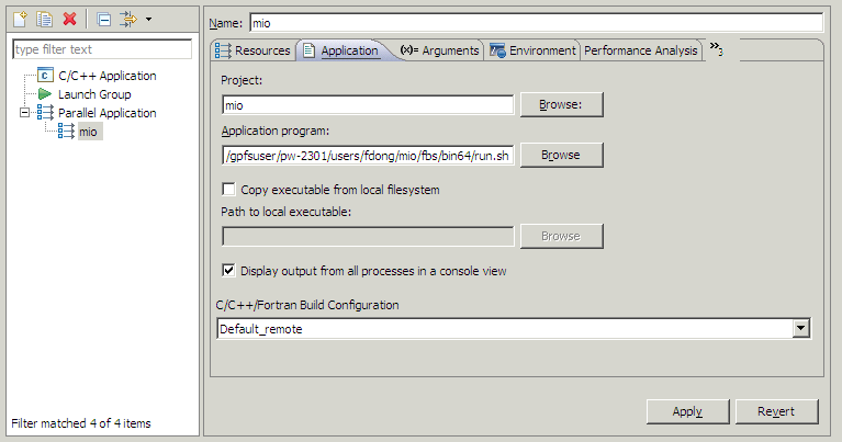
Figure 6-33 Application tab
4. Input fbs.inst as the argument for run.sh, and set the working directory as /gpfsuser/pw-2301/users/fdong/mio/fbs/bin64, as shown in Figure 6-34.

Figure 6-34 Arguments tab
5. Click Apply → Profile, after the application complete, asks Do you want to automatically open these visualization files, as shown in Figure 6-35 on page 127.

Figure 6-35 Open visualization files
6. Click Yes. The plug-in attempts to display the I/O profiling data that was collected when the application was run. You get the visualization file open in the Performance Data tab, as shown in Figure 6-36 (visualization files in the performance data tab).

Figure 6-36 Visualization files in performance data tab
The plug-in displays the data in a tree format, in which the top-level node is the file that the application read or wrote and the leaf nodes are the I/O function calls your application issued for that file. Figure 6-37 on page 128 shows the data visualization window with this tree fully expanded.

Figure 6-37 Performance data summary view with I/O profiling data
Each row shows the time spent in an I/O function call and the number of times that the function call is executed.
7. You can view detailed data for a leaf node by right-clicking over it and selecting Show Metric Browser from the pop-up menu. A metric browser window contains data for each process that executed that I/O function. You can view all of your performance measurements in a tabular form by selecting the Show Data as a Flat Table option from the pop-up menu that appears when you right-click within the Performance Data Summary view.
8. You can view a plot of your I/O measurements by right-clicking in the Performance Data Summary view, selecting Load IO Trace from the pop-up menu that appears, and specifying the location to download the I/O trace file like hpct_mio.mio.evt.iot. After the trace is loaded, the Eclipse window looks like Figure 6-38 (MIO summary).

Figure 6-38 MIO summary
The MIO Summary view contains a tree view of the MIO performance data files. The top-level nodes represent individual performance data files. The next level nodes represent individual files that the application accessed. The next level nodes represent the application program. You can select leaf nodes to include the data from those nodes in the plot window.
You can use the buttons in the view’s toolbar or the menu options in the view’s drop-down menu to perform the following actions (Table 6-10).
Table 6-10 MIO trace processing actions
|
Button
|
Action
|
|
Load MIO Trace
|
Load a new I/O trace file.
|
|
Display MIO Trace
|
Display a new I/O trace file.
|
|
Display MIO Tables
|
Display data from the I/O trace in a tabular format.
|
After you select write and read leaf nodes from the tree and click the Display MIO Trace button, the Eclipse window looks like Figure 6-39 on page 129 (MIO trace view).

Figure 6-39 MIO trace view
We can see that, the application is writing a file sequentially, after finished, read the file from beginning to the end, and then reversed. The blue line is write operation, and the red line is read operation.
When the graph is initially displayed, the Y axis represents the file position, in bytes. The X axis of the graph always represents time in seconds.
You can zoom into an area of interest in the graph by left-clicking at one corner of the desired area and dragging the mouse while holding the left button to draw a box around the area of interest and then releasing the left-mouse button. When you release the left-mouse button, the plug-in redraws the graph, showing the area of interest. You can then zoom in and out of the graph by clicking the Zoom In and Zoom Out buttons at the top of the graph window. As you drag the mouse, the plug-in displays the X and Y coordinates of the lower-left corner of the box, the upper-right corner of the box, and the slope of the line between those two corners as text in the status bar area at the bottom of the view.
You can determine the I/O data transfer rate at any area in the plot by right-clicking over the desired starting point in the plot and holding down the right-mouse button, while tracing over the section of the plot of interest. The coordinates of the starting and ending points of the selection region and the data transfer rate (slope) are displayed in the status area at the bottom of the view.
You can save the current plot to a jpeg file by clicking Save at the top of the view. A file selector dialog appears, which allows you to select the path name of the file to which the screen image will be written.
You can display a pop-up dialog that lists the colors in the current graph and the I/O functions they are associated with by clicking Show Key at the top of the view.
You can view the I/O profiling data in tabular form and modify the characteristics of the current plot by selecting Display MIO Tables at the top of the MIO Summary view. A window similar to Figure 6-40 on page 130 (dataview table view) is displayed.

Figure 6-40 DataView table view
There are four widgets at the top of the table view that you can use to modify the characteristics of the current plot. You can change the values in these widgets as desired. The selections you make in this view are effective the next time you click Display MIO Trace in the MIO Summary view.
The colored square at the upper left specifies the color to use when drawing the plot. If you click this square, a color selector dialog appears, which allows you to select the color you want to be used in drawing the plot.
The second widget from the left, labeled file position activity, selects the metric to be used for the Y and X axis of the plot and also affects the format of the plot. If you select file position activity, the Y axis represents the file position and the X axis represents time. If you select data delivery rate, the Y axis represents the data transfer rate and the X axis represents time. If you select rate versus pos, the Y axis represents the data transfer rate and the X axis represents the start position in the file.
The third widget from the left specifies the pixel width for the graph that is drawn when the file position metric is selected from the second widget from the left.
The right most widget specifies the metric that has its numeric value displayed next to each data point. You can select any column displayed in the table, or none to plot each point with no accompanying data value.
6.1.7 X Windows Performance Profiler
The X Windows Performance Profiler (Xprof) is a fronted tool for profiling data generated by running an application that was compiled and linked with the -pg option. It assists in identifying most CPU-Intensive functions in parallel applications. It comes with the IBM HPC Toolkit, although it is not currently integrated within Eclipse. As a consequence, the tool must be started in the target system manually and exported to the graphical view using either X-forwarding or VNC techniques.
Preparing your application
The parallel application must be compiled using the -pg flag. Optionally, it can also be compiled with -g flag so that Xprof can get the connection to the line of source code.
Profiling with Xprof
To profile with Xprof:
1. Compile the application using the -pg option.
2. Run the application to generate gmon.out profile data files.
3. Open the Xprof GUI passing the binary and gmon.out files as arguments (Example 6-4). Optionally you can just start Xprof without arguments and then select File → Load Files to select and load the required files.
Example 6-4 Starting Xprof GUI on Linux
$ source /opt/ibmhpc/ppedev.hpct/env_sh
$ Xprof ./Gadget2 profdir.0_0/gmon.out profdir.0_1/gmon.out
Observe that gmon.out files are generated with different names in Linux and AIX operating systems, respectively, profdir.<world_id>_<task_id>/gmon.out and gmon.<world_id>_<task_id>.out.
Interpreting profile information
After binary and profile files are loaded, the main panel is going to display a call graph chart of application execution for a consolidated visualization of all data collected (Figure 6-41 on page 132). In that chart, nodes are application methods and arcs are method calls, so a pair of node-arc represents the caller/callee relationship at runtime. The rectangles embodying a node represents time spent in a method and its callees, with a representation of time spent in the method itself plus its callees and height represents the time spent only in that method.
It is also possible to do several operations in the call graph main view, such as:
•Apply filters to cluster or uncluster methods (menu Filter → uncluster Function).
•Access detailed information about each function (right click in a rectangle).
•Access detailed information about specific caller/callee flow, including the number of times that pair was executed (right-click in an arc).
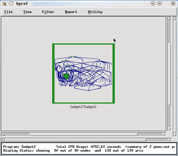
Figure 6-41 Xprof main window: call graph
The tool supports several visualization modes and reports that are accessible from the Reports menu. It is also possible to navigate from a report back (and fourth) to the call graph view. Some of the available reports are:
•Flat profile report
•Call graph (plain text) report
•Function call statistics report
•Library statistics report
Indeed those reports are rich and useful to easily identify hotspots in the source code, for example, the flat profile report sorts out the application functions by accumulated time spent in each one, thus highlighting the most CPU-intensive on the top (Figure 6-42 on page 133).
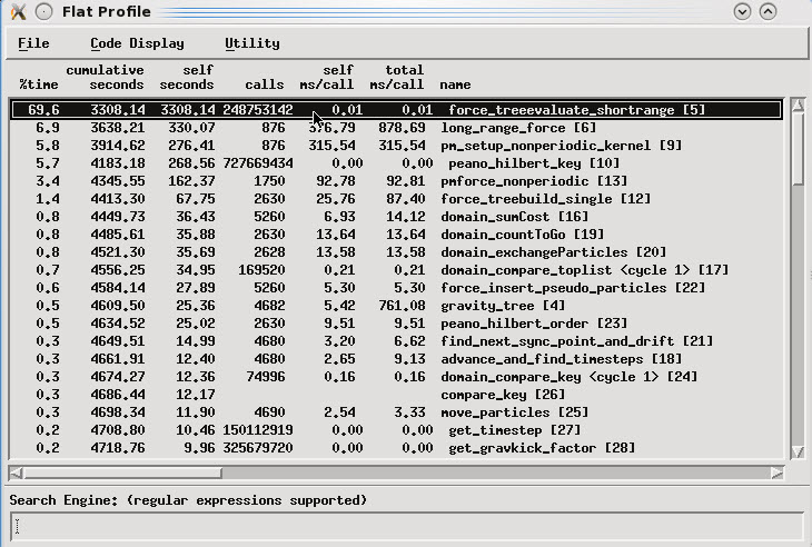
Figure 6-42 Xprof: flat profile report
6.2 Debugging
This section provides debugging information.
6.2.1 Parallel Static Analysis
The IBM Parallel Environment (PE) Developer Edition comes with a set of tools for static analysis of parallel application source code. They can show artifacts and make analysis for the parallel technologies shown in Table 6-11.
Table 6-11 Parallel static analysis capabilities versus parallel technologies
|
Technology
|
Show artifacts
|
Analysis
|
|
MPI
|
Yes
|
Yes
|
|
OpenMP
|
Yes
|
No
|
|
LAPI
|
Yes
|
No
|
|
OpenACC
|
Yes
|
No
|
|
OpenSHMEM
|
Yes
|
No
|
|
PAMI
|
Yes
|
No
|
|
UPC
|
Yes
|
No
|
Any of the parallel static analyze tools of Table 6-11 are executed from the drop-down menu in the Eclipse toolbar, as shown in Figure 6-43 on page 134.

Figure 6-43 Parallel static analysis menu
The tool scan the project files to gather data and then generate reports with artifact types (Figure 6-44) being used and their exact location in the source code, as shown in Figure 6-45.

Figure 6-44 Parallel analysis message displayed after finish analysis

Figure 6-45 Parallel analysis report view for MPI project
If the tools cannot find the artifacts in your source code, some additional configuration might be needed on Eclipse. For OpenMP artifacts, select Window → Preferences and choose Parallel Tools → Parallel Language Development Tools → OpenMP. Make sure to enable the option Recognize OpenMP Artifacts by prefix (omp_) alone?, and add the OpenMP include paths of your local system. If you do not have the OpenMP include files in your local system, you can add any path (for example, the path to the project on your workspace). Figure 6-46 on page 135 shows the screen used for OpenMP artifacts configuration.

Figure 6-46 OpenMP artifacts configuration
To be able to identify the UPC artifacts, a similar configuration might be needed as well. Go to menu Window → Preferences, and choose Parallel Tools → Parallel Language Development Tools → UPC. Make sure to enable the option Recognize APIs by prefix (upc_) alone?, and add the UPC include paths of your local system. If you do not have the UPC include files in your local system, you can add any path (for example, the path to the project on your workspace). Figure 6-47 on page 136 shows the screen used for UPC artifacts configuration.

Figure 6-47 UPC artifacts configuration
If your project uses Fortran code and the parallel artifacts were still not recognized, change the configuration regarding how Eclipse handles the source form of your Fortran source files. Select your project on the Project Explorer view, select File → Properties, and choose Fortran General → Source Form. On this screen, change the source form for the *.F and *.f file extensions to Fixed Form - INCLUDE lines ignored, as shown in Figure 6-48 on page 137.
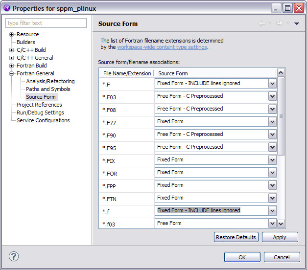
Figure 6-48 Fortran source form configuration
MPI barrier analysis
This tool can generate statistics about MPI artifacts and also assist with identify barrier problems while implementing a parallel application. The tools makes the following analysis across multiple source files:
•Potential deadlocks
•Barrier matches
•Barrier synchronization errors
Figure 6-49 shows the barrier matches report that assist to browse through the MPI barriers in your source code.

Figure 6-49 MPI analysis: barrier matches report
If any barrier problem is found during the analysis, a message is displayed, as shown in Figure 6-50. The MPI Barrier Errors view is opened, displaying the barrier errors report shown in Figure 6-51. This view can also be used to easily find the line on the source code where the problems was found.
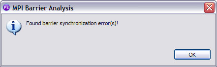
Figure 6-50 MPI barrier error found
Figure 6-51 MPI analysis: barrier error report
6.2.2 Eclipse PTP Parallel debugger
This section describes basic procedures to use the eclipse built-in parallel debugger and state differences to the single process (or thread) one. For further details regarding this topic, we suggest you consult the PTP parallel debugger help, accessible through Eclipse menu bar (Help → Help Contents → Parallel Tools Platform (PTP) User Guide → Parallel Debugging).
The parallel debugger provides some specific debugging features for parallel applications that distinguish it from Eclipse debugger for serial applications. In particular, it is designed to threat parallel application as a set of processes, allowing a group to:
•Visualize their relationships with jobs
•Enable their management
•Apply common debugging operations
Debugging is still based on the breakpoint concept, but here it provides a special type known as a parallel breakpoint, also designed to operate in a set rather than a single process (or thread). There are two types of parallel breakpoints:
•Global breakpoints: Apply to all processes in any job
•Local breakpoints: Apply only to a specific set of processes for a single job
The current instruction pointer is also particular for parallel applications in the sense that:
•It shows one instruction pointer for every group of processes at the same location.
•The group of processes represented by an instruction pointer is not necessarily the same as a process set; therefore, different markers are used to indicate the types of processes stopped at a given location.
The parallel debugger relies on a server-side agent called Scalable Debug Manager (SDM) that is in charge of controlling the debug session. You need to properly set its path at the Debugger tab in the new debug launcher configuration window (Figure 6-52).
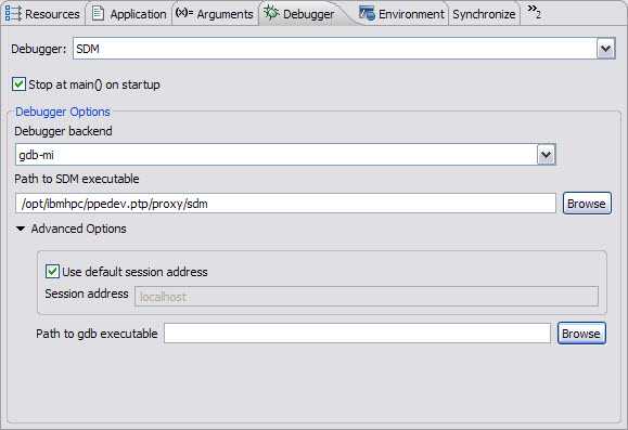
Figure 6-52 Debug launcher configuration: Debugger tab
1 Do not mix different modes because they will affect each other. Any calls to instrumentation functions that you code in your application (code instrumentation) might interfere with the instrumentation calls that are inserted by the toolkit (binary instrumentation).
2 Not supported in x86 Linux systems.
3 IBM HPC Toolkit binary instrumentation will operate reliably on executables with a text segment size of no more than 32 MB.
..................Content has been hidden....................
You can't read the all page of ebook, please click here login for view all page.