

Storage back-end
This chapter describes the aspects and practices to consider when system’s external back-end storage is planned, configured, and managed.
External storage is acquired by Spectrum Virtualize by virtualizing a separate IBM or third-party storage system, which are attached with FC or iSCSI.
|
Note: IBM SAN Volume Controller that is built on SV1 nodes supports SAS-attached expansions with solid-state drives (SSDs) and hard disk drives (HDDs). However, nodes SV2 and SA2 do not support internal storage.
For more information about configuring internal storage that is attached to SV1 nodes, see IBM FlashSystem Best Practices and Performance Guidelines, SG24-8503.
|
This chapter includes the following topics:
3.1 General considerations for managing external storage
IBM SAN Volume Controller can virtualize external storage that is presented to the system. External back-end storage systems (or controllers in Spectrum Virtualize terminology) provide their logical volumes (LVs), which are detected by IBM SAN Volume Controller as MDisks and can be used in storage pools.
This section covers aspects of planning and managing external storage that is virtualized by IBM SAN Volume Controller.
External back-end storage can be connected to IBM SAN Volume Controller with FC (SCSI) or iSCSI. NVMe-FC back-end attachment is not supported because it provides no performance benefits for IBM SAN Volume Controller. The main advantage of NVMe solution is seen as a reduction in the CPU cycles that are needed on the host level, where the Fibre Channel HBA is found, to handle the interrupts.
For external backend, IBM SAN Volume Controller acts as a host. All Spectrum Virtualize Fibre Channel drivers are implemented from day one as polling drivers, not interrupt-driven drivers. Thus, on the storage side, almost no latency savings are gained by switching from SCSI to NVMe as a protocol.
3.1.1 Storage controller path selection
When a managed disk (MDisk) logical unit (LU) is accessible through multiple storage system ports, the system ensures that all nodes that access this LU coordinate their activity and access the LU through the same storage system port.
An MDisk path that is presented to the storage system for all system nodes must meet the following criteria:
•The system node:
– Is a member of a storage system
– Includes Fibre Channel or iSCSI connections to the storage system port
– Successfully discovered the LU
•The port selection process did not cause the system node to exclude access to the MDisk through the storage system port
When the IBM SAN Volume Controller node selects a set of ports to access the storage system, the two types of path selection that are described in the next sections are supported to access the MDisks. A type of path selection is determined by external system type and cannot be changed.
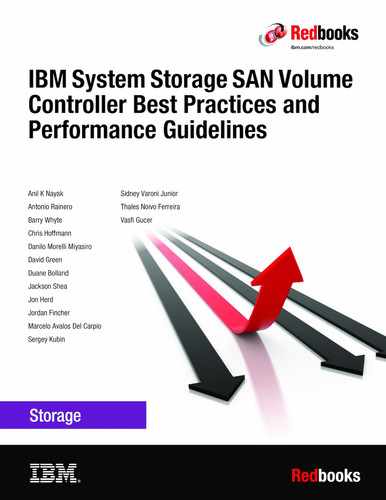
To determine which algorithm is used for a specific back-end system, see System Storage Interoperation Center (SSIC), as shown in Figure 3-1.

Figure 3-1 SSIC example
Round-robin path algorithm
With the round-robin path algorithm, each MDisk uses one path per target port per IBM SAN Volume Controller node. Therefore, in cases of storage systems that do not feature a preferred controller (such as XIV or DS8000), each MDisk uses all of the available FC ports of that storage controller.
With a round-robin compatible storage controller, there is no need to create as many volumes as there are storage FC ports. Every volume, and therefore MDisk, uses all available IBM SAN Volume Controller ports.
This configuration results in a significant performance increase because the MDisk is no longer bound to one back-end FC port. Instead, it can issue I/Os to many back-end FC ports in parallel. Particularly, the sequential I/O within a single extent can benefit from this feature.
Additionally, the round-robin path selection improves resilience to specific storage system failures. For example, if one of the back-end storage system FC ports encounters some performance problems, the I/O to MDisks is sent through other ports. Moreover, because I/Os to MDisks are sent through all back-end storage FC ports, the port failure can be detected more quickly.
|
Preferred practice: If your storage system supports the round-robin path algorithm, zone as many FC ports from the back-end storage controller as possible. IBM SAN Volume Controller supports up to 16 FC ports per storage controller. For more information about FC port connections and zoning guidelines, see your storage system documentation.
|
Example 3-1 shows a storage controller that supports round-robin path selection.
Example 3-1 Round robin enabled storage controller
IBM_2145:SVC-ITSO:superuser>lsmdisk 4
id 4
name mdisk4
...
preferred_WWPN
active_WWPN many ? <<< Round Robin Enabled
MDisk group balanced and controller balanced
Although round-robin path selection provides optimized and balanced performance with minimum configuration required, some storage systems still require manual intervention to achieve the same goal.
With storage subsystems, such as IBM DS5000 and DS3000 (or other Active-Passive type systems), IBM SAN Volume Controller accesses an MDisk LU through one of the ports on the preferred controller. To best use the back-end storage, it is important to ensure that the number of LUs that is created is a multiple of the connected FC ports and aggregate all LUs to a single MDisk group.
Example 3-2 shows a storage controller that supports MDisk group balanced path selection.
Example 3-2 MDisk group balanced path selection (no round robin enabled) storage controller
IBM_2145:SVC-ITSO:superuser>lsmdisk 5
id 5
name mdisk5
...
preferred_WWPN
active_WWPN 20110002AC00C202 ? <<< indicates MDisk group balancing
3.1.2 Guidelines for creating optimal back-end configuration
Most of the back-end controllers aggregate spinning or SSDs into RAID arrays, then join arrays into pools. Logical volumes are created on those pools and provided to hosts.
When connected to external back-end storage, IBM SAN Volume Controller acts as a host. It is important to create back-end controller configuration that provides performance and resiliency because IBM SAN Volume Controller relies on back-end storage when serving I/O to host systems that are attached to it.
If your back-end system includes homogeneous storage, create the required number of RAID arrays (usually RAID 6 or RAID 10 are recommended) with an equal number of drives. The type and geometry of array depends on the back-end controller vendor’s recommendations. If your back-end controller can spread the load stripe across multiple arrays in a resource pool (for example, by striping), create a single pool and add all arrays there.
On back-end systems with mixed drives, create a separate resource pool for each drive technology (and keep drive technology type in mind because you must assign the correct tier for an MDisk when it is used by IBM SAN Volume Controller).
Create a set of fully allocated logical volumes from the back-end system storage pool (or pools). Each volume is detected as MDisk on IBM SAN Volume Controller. The number of logical volumes to create depends the type of drives that are used by your back-end controller.
Back-end controller with spinning drives
If your backend uses spinning drives, volume number calculation must be based on a queue depth. Queue depth is the number of outstanding I/O requests of a device.
For optimal performance, spinning drives need 8 - 10 concurrent I/O at the device, and this need does not change with drive rotation speed. Therefore, we want to ensure that in a highly loaded system, any IBM SAN Volume Controller MDisk can queue up approximately 8 I/O per back-end system drive.
IBM FlashSystem queue depth per MDisk is approximately 60 (the exact maximum that is seen on a real system can vary, depending on the circumstances; however, for the purpose of this calculation, it does not matter). This queue depth per MDisk number leads to the HDD Rule of 8. According to this rule, to achieve 8 I/O per drive and with queue depth 60 per MDisk from IBM FlashSystem, a back-end array with 60/8 = 7.5 that is approximately equal to eight physical drives is optimal, or we need one logical volume per every eight drives in an array
Example 1
Consider the following example:
•The backend controller to be virtualized is IBM Storwize V5030 with 64 NL-SAS 8 TB drives.
•The system is homogeneous.
•According to recommendations that are described in the “Array Considerations” section in Implementing the IBM FlashSystem with IBM Spectrum Virtualize V8.4, SG24-8465, a single DRAID6 array is created at Storwize and installed in a storage pool.
•The HDD rule of 8 tells us that we want 64/8 = 8 MDisks. Therefore, eight volumes are created from a pool to present to IBM SAN Volume Controller and then are assigned to the nearline tier.
All-flash back-end controllers
For All-Flash controllers, the considerations are more of I/O distribution across IBM SAN Volume Controller ports and processing threads than of queue depth per drive. Because most all-flash arrays that are put behind the virtualizer include high I/O capabilities, we want to make sure that we are giving IBM SAN Volume Controller the optimal chance to spread the load and evenly make use of its internal resources so that queue depths are less of a concern (because of the lower latency per I/O).
For all-flash back-end arrays, IBM recommends creating 32 logical volumes from the array capacity. By doing so, the queue depths can be kept high enough and the work is spread across the virtualizer resources.
For smaller set ups with a low number of SSDs, this number can be reduced to 16 logical volumes (which results in 16 MDisks) or even eight volumes.
Example 2
Consider the following example:
•Backend controllers to be virtualized are IBM FlashSystem 5030 with 24 Tier1 7.6 TB drives IBM FlashSystem 900.
•Virtualizer needs a pool with two storage tiers.
•On IBM FlashSystem 5030, a single DRAID6 array is created and then added to a storage pool.
•Using this all-flash rule, 32 volumes are created to present as MDisks. However, because it is small setup, the number of volumes is reduced to 16.
•On IBM FlashSystem 900, all micro-latency modules are joined into a RAID5 array and added to a storage pool. FlashSystem 900 is Tier0 solution; therefore, the all-flash rule is used and 32 volumes are created to present as MDisks.
•On virtualizer, 16 MDisks are added from IBM FlashSystem 5030 as Tier1 flash, and 32 MDisks as Tier0 flash, to a single multitier pool.
Large setup considerations
For controllers, such as IBM DS8000 and XIV, you can use all-flash rule of 32. However, with installations involving such kinds of back-end controllers, it might be necessary to consider a maximum queue depth per back-end controller port, which is set to 1000 for most supported high-end storage systems.
With high-end controllers, queue depth per MDisk can be calculated by using the following formula:
Q = ((P x C) / N) / M
Where:
Q Calculated queue depth for each MDisk
P Number of back-end controller host ports (unique WWPNs) that are zoned to IBM SAN Volume Controller (minimum is 2 and maximum is 16)
C Maximum queue depth per WWPN, which is 1000 for controllers, such as XIV or DS8000
N Number of nodes in the IBM SAN Volume Controller cluster (2, 4, 6, or 8)
M Number of volumes that are presented by back-end controller and detected as MDisks
Because we know that we want to achieve Q = 60, we can calculate the number of volumes that we need to create as:
M = (P x C) / (N x Q) ? (16 x P) / N
Example 3
A 4-node IBM SAN Volume Controller is used with 12 host ports on the IBM XIV System.
By using the Q = ((P x C) / N) / M formula, we must create M = (16 x 12)/4 = 48 volumes on IBM XIV to obtain balanced, high-performing configuration.
3.1.3 Considerations for compressing and deduplicating back-end
IBM SAN Volume Controller supports over-provisioning on selected back-end controllers. Therefore, if back-end storage performs data deduplication or data compression on LUs provisioned from it, they still can be used as external MDisks on IBM SAN Volume Controller.
The implementation steps for thin-provisioned MDisks are the same as for fully allocated storage controllers. Extreme caution should be used when planning capacity for such configurations.
IBM SAN Volume Controller detects if the MDisk is thin-provisioned, its total physical capacity that is used, and remaining physical capacity. It also detects if SCSI UNMAP commands are supported by the back-end.
By sending SCSI UNMAP commands to thin-provisioned MDisks, the system marks data that is no longer used. Then, the garbage collection processes on the backend can free unused capacity and reallocate it to free space.
The use of a suitable compression or data deduplication ratio is key to achieving a stable environment. If you are unsure about the real compression or data deduplication ratio, contact your IBM technical sales representative for more information.
The nominal capacity from a compression and deduplication enabled storage system is not fixed and it varies based on the nature of the data. Always use a conservative data reduction ratio for the initial configuration.
The use of an incorrect ratio for capacity assignment can cause an out of space situation. If the MDisks do not provide enough capacity, IBM SAN Volume Controller disables access to all the volumes in the storage pool, as shown in the following example:
•Assumption 1: Sizing is performed with an optimistic 5:1 rate
•Assumption 2: Real rate is 3:1
•Physical Capacity: 20 TB
•Calculated capacity: 20 TB x 5 = 100 TB
•Volume assigned from compression or deduplication enabled storage subsystem to SAN Volume Controller or Storwize: 100 TB
•Real usable capacity: 20 TB x 3 = 60 TB
If the hosts try to write more than 60 TB data to the storage pool, the storage subsystem cannot provide any more capacity. All volumes that are used as IBM Spectrum Virtualize or Storwize Managed Disks and all related pools go offline.
Thin-provisioned back-end storage must be carefully monitored. It is necessary to set up capacity alerts to be aware of the real remaining physical capacity.
Also, the best practice is to have an emergency plan for “Out Of Physical Space” situation on the back-end controller to know what steps must be taken to recover. The plan also must be prepared during the initial implementation phase.
3.2 Controller-specific considerations
This section discusses implementation information that is related to supported back-end systems. For more information about general requirements, see IBM Documentation.
3.2.1 Considerations for DS8000 series
In this section, we discuss considerations for the DS800 series.
Interaction between DS8000 and IBM SAN Volume Controller
It is important to know DS8000 drive virtualization process; that is, the process of preparing physical drives for storing data that belongs to a volume that is used by a host (in this case, the IBM SAN Volume Controller).
In this regard, the basis for virtualization begins with the physical drives of DS8000, which are mounted in storage enclosures. Virtualization builds upon the physical drives as a series of the following layers:
•Array sites
•Arrays
•Ranks
•Extent pools
•Logical volumes
•Logical subsystems
Array sites are the building blocks that are used to define arrays, which are data storage systems for block-based, file-based, or object based storage. Instead of storing data on a server, storage arrays use multiple drives that are managed by a central management and can store a huge amount of data. In general terms, eight identical drives that have the same capacity, speed, and drive class are called the array site. When an array is created, the RAID level, array type, and array configuration are defined. RAID 5, RAID 6, and RAID 10 levels are supported.
|
Important: Normally, the RAID 6 is highly preferred and is the default while the Data Storage Graphical Interface (DS GUI) is used. As with large drives in particular, the RAID rebuild times (after one drive failure) get ever larger. The use of RAID 6 reduces the danger of data loss because of a double-RAID failure. For more information, see IBM Documentation.
|
A rank, which is a logical representation for the physical array, is relevant for an IBM SAN Volume Controller because of the creation of fixed block (FB) pool for each array that you want to virtualize. Ranks in DS8000 are defined in a one-to-one relationship to arrays. It is for this reason that a rank is defined as using only one array.
A fixed block rank that features an extent size of 1 GiB is a large extent; an extent size of 16 MiB is a small extent.
An extent pool or storage pool in DS8000 is a logical construct to add the extents from a set of ranks, which forms a domain for extent allocation to a logical volume.
In synthesis, a logical volume consists of a set of extents from one extent pool or storage pool. DS8900F supports up to 65,280 logical volumes.
A logical volume that is composed of fix block extents is called LUN. A fix block LUN consist of one or more 1 GiB (large) extents, or one or more 16 MiB (small) extents from one FB extent pool. Although a LUN cannot cross extent pools, it can have extents from multiple ranks within the same extent pool.
|
Important: DS8000 Copy Services do not support FB logical volumes larger than 2 TiB. Do not create a LUN that is larger than 2 TiB if you want to use Copy Services for the LUN unless the LUN is integrated as Managed Disks in an IBM FlashSystem. Use IBM Spectrum Virtualize Copy Services instead. Based on the considerations, the following maximum LUN sizes are used to create at DS8900F and present to IBM FlashSystem:
•16 TB LUN with large extents (1 GiB)
•16 TB LUN with small extent (16 MiB) for DS8880F with version or edition R8.5 or later, and for DS8900F R9.0 or later
|
Logical subsystems (or LSS) are another logical construct, and mostly used with fixed block volumes. Thus, 255 LSSs as a maximum can exist on DS8900F. For more information, see IBM Documentation.
The concepts of virtualization of DS8900F for IBM FlashSystem or IBM SAN Volume Controller are shown in Figure 3-2.

Figure 3-2 DS8900 virtualization concepts focus to IBM SAN Volume Controller
Connectivity considerations
The number of DS8000 ports to be used is at least eight. With large and workload intensive configurations, consider using up to 16 ports, which is the maximum that is supported by IBM SAN Volume Controller.
Generally, use ports from different host adapters and, if possible, from different I/O enclosures. This configuration is also important because during a DS8000 LIC update, a host adapter port might need to be taken offline. This configuration allows the IBM SAN Volume Controller I/O to survive a hardware failure on any component on the SAN path.
For more information about SAN preferred practices and connectivity, see Chapter 2, “Storage area network” on page 19.
Defining storage
To optimize the DS8000 resource usage, use the following guidelines:
•Distribute capacity and workload across device adapter pairs.
•Balance the ranks and extent pools between the two DS8000 internal servers to support the corresponding workloads on them.
•Spread the logical volume workload across the DS8000 internal servers by allocating the volumes equally on rank groups 0 and 1.
•Use as many disks as possible. Avoid idle disks, even if all storage capacity is not to be used initially.
•Consider the use of multi-rank extent pools.
•Stripe your logical volume across several ranks (the default for multi-rank extent pools).
Balancing workload across DS8000 series controllers
When you configure storage on the DS8000 series disk storage subsystem, ensure that ranks on a device adapter (DA) pair are evenly balanced between odd and even extent pools. If you do not ensure that the ranks are balanced, uneven device adapter loading can lead to a considerable performance degradation.
The DS8000 series controllers assign server (controller) affinity to ranks when they are added to an extent pool. Ranks that belong to an even-numbered extent pool have an affinity to server0, and ranks that belong to an odd-numbered extent pool have an affinity to server1.
Figure 3-3 on page 77 shows an example of a configuration that results in a 50% reduction in available bandwidth. Notice how arrays on each of the DA pairs are accessed only by one of the adapters. In this case, all ranks on DA pair 0 are added to even-numbered extent pools, which means that they all have an affinity to server0. Therefore, the adapter in server1 is sitting idle. Because this condition is true for all four DA pairs, only half of the adapters are actively performing work. This condition can also occur on a subset of the configured DA pair.

Figure 3-3 DA pair reduced bandwidth configuration
Example 3-3 shows what this invalid configuration resembles from the CLI output of the lsarray and lsrank commands. The arrays that are on the same DA pair contain the same group number (0 or 1), meaning that they have affinity to the same DS8000 series server. Here, server0 is represented by group0, and server1 is represented by group1.
As an example of this situation, consider arrays A0 and A4, which are attached to DA pair 0. In this example, both arrays are added to an even-numbered extent pool (P0 and P4) so that both ranks have affinity to server0 (represented by group0), which leaves the DA in server1 idle.
Example 3-3 Command output for the lsarray and lsrank commands
dscli> lsarray -l
Date/Time: Oct 20, 2016 12:20:23 AM CEST IBM DSCLI Version: 7.8.1.62 DS: IBM.2107-75L2321
Array State Data RAID type arsite Rank DA Pair DDMcap(10^9B) diskclass
===================================================================================
A0 Assign Normal 5 (6+P+S) S1 R0 0 146.0 ENT
A1 Assign Normal 5 (6+P+S) S9 R1 1 146.0 ENT
A2 Assign Normal 5 (6+P+S) S17 R2 2 146.0 ENT
A3 Assign Normal 5 (6+P+S) S25 R3 3 146.0 ENT
A4 Assign Normal 5 (6+P+S) S2 R4 0 146.0 ENT
A5 Assign Normal 5 (6+P+S) S10 R5 1 146.0 ENT
A6 Assign Normal 5 (6+P+S) S18 R6 2 146.0 ENT
A7 Assign Normal 5 (6+P+S) S26 R7 3 146.0 ENT
dscli> lsrank -l
Date/Time: Oct 20, 2016 12:22:05 AM CEST IBM DSCLI Version: 7.8.1.62 DS: IBM.2107-75L2321
ID Group State datastate Array RAIDtype extpoolID extpoolnam stgtype exts usedexts
======================================================================================
R0 0 Normal Normal A0 5 P0 extpool0 fb 779 779
R1 1 Normal Normal A1 5 P1 extpool1 fb 779 779
R2 0 Normal Normal A2 5 P2 extpool2 fb 779 779
R3 1 Normal Normal A3 5 P3 extpool3 fb 779 779
R4 0 Normal Normal A4 5 P4 extpool4 fb 779 779
R5 1 Normal Normal A5 5 P5 extpool5 fb 779 779
R6 0 Normal Normal A6 5 P6 extpool6 fb 779 779
R7 1 Normal Normal A7 5 P7 extpool7 fb 779 779
Figure 3-4 shows a configuration that balances the workload across all four DA pairs.

Figure 3-4 DA pair correct configuration
Figure 3-5 shows what a correct configuration resembles the CLI output of the lsarray and lsrank commands. Notice that the output shows that this configuration balances the workload across all four DA pairs with an even balance between odd and even extent pools. The arrays that are on the same DA pair are split between groups 0 and 1.

Figure 3-5 The lsarray and lsrank command output
DS8000 series ranks to extent pools mapping
In the DS8000 architecture, extent pools are used to manage one or more ranks. An extent pool is visible to both processor complexes in the DS8000 storage system, but it is directly managed by only one of them. You must define a minimum of two extent pools with one extent pool that is created for each processor complex to fully use the resources. You can use the following approaches:
•One-to-one approach: One rank per extent pool configuration
With this approach, DS8000 is formatted in 1:1 assignment between ranks and extent pools. This configuration disables any DS8000 storage pool striping or auto-rebalancing activity, if it is enabled. You can create one or two volumes in each extent pool exclusively on one rank only and put all of those volumes into one IBM SAN Volume Controller storage pool. SAN Volume| Controller stripes across all of these volumes and balances the load across the RAID ranks by that method. No more than two volumes per rank are needed with this approach. Therefore, the rank size determines the volume size.
Systems often are configured with at least two storage pools: One (or two) containing MDisks of all the 6+P RAID 5 ranks of the DS8000 storage system, and the other one (or more) containing the slightly larger 7+P RAID 5 ranks. This approach maintains equal load balancing across all ranks when the IBM SAN Volume Controller striping occurs because each MDisk in a storage pool is the same size.
The IBM SAN Volume Controller extent size is the stripe size that is used to stripe across all these single-rank MDisks.
This approach delivered good performance and has its justifications. However, it also includes a few minor drawbacks. A natural skew can exist, such as a small file of a few hundred KiB that is heavily accessed. When you have more than two volumes from one rank, but not as many IBM SAN Volume Controller storage pools, the system might start striping across many entities that are effectively in the same rank, depending on the storage pool layout. Such striping should be avoided.
An advantage of this approach is that it delivers more options for fault isolation and control over where a specific volume and extent are located.
•Many-to-one approach: Multi-rank extent pool configuration
A more modern approach is to create a few DS8000 extent pools; for example, two DS8000 extent pools. Use DS8000 storage pool striping or automated Easy Tier rebalancing to help prevent from overloading individual ranks.
Create at least two extent pools for each tier to balance the extent pools by Tier and Controller affinity. Mixing different tiers on the same extent pool is effective only when Easy Tier is activated on the DS8000 pools. However, when virtualized, tier management has more advantages when handled by the IBM SAN Volume Controller. For more information about choosing which level to run Easy Tier, see “External controller tiering considerations” on page 167.
You need only one volume size with this multi-rank approach because enough space is available in each large DS8000 extent pool. The maximum number of back-end storage ports to be presented to the IBM SAN Volume Controller is 16. Each port represents a path to the IBM SAN Volume Controller. Therefore, when sizing the number of LUN/MDisks to be presented to the IBM SAN Volume Controller, the suggestion is to present at least 2 - 4 volumes per path. Therefore, using the maximum of 16 paths, create 32, 48, or 64 DS8000 volumes, which maintains a good queue depth for this configuration.
To maintain the highest flexibility and for easier management, large DS8000 extent pools are beneficial. However, if the DS8000 installation is dedicated to shared-nothing environments, such as Oracle ASM, IBM DB2® warehouses, or General Parallel File System (GPFS), use the single-rank extent pools.
LUN masking
For a storage controller, all IBM SAN Volume Controller nodes must detect the same set of LUs from all target ports that logged in. If target ports are visible to the nodes or canisters that do not have the same set of LUs assigned, IBM SAN Volume Controller treats this situation as an error condition and generates error code 1625.
You must validate the LUN masking from the storage controller and then, confirm the correct path count from within the IBM SAN Volume Controller.
The DS8000 series controllers perform LUN masking that is based on the volume group. Example 3-4 shows the output of the showvolgrp command for volume group (V0), which contains 16 LUNs that are being presented to a two-node IBM SAN Volume Controller cluster.
Example 3-4 Output of the showvolgrp command
dscli> showvolgrp V0
Date/Time: Oct 20, 2016 10:33:23 AM BRT IBM DSCLI Version: 7.8.1.62 DS: IBM.2107-75FPX81
Name ITSO_SVC
ID V0
Type SCSI Mask
Vols 1001 1002 1003 1004 1005 1006 1007 1008 1101 1102 1103 1104 1105 1106 1107 1108
Example 3-5 shows output for the lshostconnect command from the DS8000 series. In this example, you can see that four ports of the two-node cluster are assigned to the same volume group (V0) and therefore, are assigned to the same four LUNs.
Example 3-5 Output for the lshostconnect command
dscli> lshostconnect -volgrp v0
Date/Time: Oct 22, 2016 10:45:23 AM BRT IBM DSCLI Version: 7.8.1.62 DS: IBM.2107-75FPX81
Name ID WWPN HostType Profile portgrp volgrpID ESSIOport
=============================================================================================
ITSO_SVC_N1C1P4 0001 500507680C145232 SVC San Volume Controller 1 V0 all
ITSO_SVC_N1C2P3 0002 500507680C235232 SVC San Volume Controller 1 V0 all
ITSO_SVC_N2C1P4 0003 500507680C145231 SVC San Volume Controller 1 V0 all
ITSO_SVC_N2C2P3 0004 500507680C235231 SVC San Volume Controller 1 V0 all
From Example 3-5, you can see that only the IBM SAN Volume Controller WWPNs are assigned to V0.
|
Attention: Data corruption can occur if the same LUN is assigned to IBM SAN Volume Controller nodes and other devices, such as hosts attached to DS8000.
|
Next, you see how the IBM SAN Volume Controller detects these LUNs if the zoning is properly configured. The Managed Disk Link Count (mdisk_link_count) represents the total number of MDisks that are presented to the IBM SAN Volume Controller cluster by that specific controller.
Example 3-6 shows the general details of the output storage controller by using the system CLI.
Example 3-6 Output of the lscontroller command
IBM_2145:SVC-ITSO:superuser>svcinfo lscontroller DS8K75FPX81
id 1
controller_name DS8K75FPX81
WWNN 5005076305FFC74C
mdisk_link_count 16
max_mdisk_link_count 16
degraded no
vendor_id IBM
product_id_low 2107900
...
WWPN 500507630500C74C
path_count 16
max_path_count 16
WWPN 500507630508C74C
path_count 16
max_path_count 16
IBM SAN Volume Controller MDisks and storage pool considerations
The recommended practice is to create a single IBM SAN Volume Controller storage pool per DS8900F system. This configuration simplifies management, and increases overall performance.
An example of preferred configuration is shown in Figure 3-6. Four Storage pools or Extent pools (one even and one odd) of DS8900F are joined into one IBM SAN Volume Controller storage pool.

Figure 3-6 Four DS8900F extent pools as one IBM SAN Volume Controller storage pool
To determine how many logical volumes must be created to present to IBM SAN Volume Controller as MDisks, see 3.1.2, “Guidelines for creating optimal back-end configuration” on page 70.
3.2.2 IBM XIV Storage System considerations
XIV Gen3 volumes can be provisioned to IBM SAN Volume Controller by way of iSCSI and FC. However, it is preferred to implement FC attachment for performance and stability considerations, unless a dedicated IP infrastructure for storage is available.
Host options and settings for XIV systems
You must use specific settings to identify IBM SAN Volume Controller systems as hosts to XIV systems. An XIV node within an XIV system is a single WWPN.
An XIV node is considered to be a single SCSI target. Each host object that is created within the XIV System must be associated with the same LUN map.
From an IBM SAN Volume Controller perspective, an XIV Type Number 281x controller can consist of more than one WWPN. However, all are placed under one worldwide node number (WWNN) that identifies the entire XIV system.
Creating a host object for IBM SAN Volume Controller for an IBM XIV
A single host object with all WWPNs of IBM SAN Volume Controller nodes can be created when implementing IBM XIV. This technique makes the host configuration easier to configure. However, the ideal host definition is to consider each node IBM SAN Volume Controller as a host object, and create a cluster object to include all nodes or canisters.
When implemented in this manner, statistical metrics are more effective because performance can be collected and analyzed on IBM SAN Volume Controller node level.
For more information about creating a host on XIV, see IBM XIV Gen3 with IBM System Storage SAN Volume Controller and Storwize V7000, REDP-5063.
Volume considerations
As modular storage, XIV storage can be presented 6 - 15 modules in a configuration. Each module that is added to the configuration increases the XIV capacity, CPU, memory, and connectivity. The XIV system currently supports the following configurations:
•28 - 81 TB when 1 TB drives are used
•55 - 161 TB when 2 TB disks are used
•84 - 243 TB when 3 TB disks are used
•112 - 325 TB when 4 TB disks are used
•169 - 489 TB when 6 TB disks are used
Figure 3-7 shows how XIV configuration varies according to the number of modules present on the system.

Figure 3-7 XIV rack configuration: 281x-214
Although XIV has its own queue depth characteristics for direct host attachment, the best practices that are described in 3.1.2, “Guidelines for creating optimal back-end configuration” on page 70 are preferred when you virtualize XIV with IBM Spectrum Virtualize.
Suggested volume sizes and quantities for IBM SAN Volume Controller on the XIV systems with different drive capacities are listed in Table 3-1.
Table 3-1 XIV minimum volume size and quantity recommendations
|
Modules
|
XIV
host ports |
Volume
size (GB)
1 TB drives |
Volume
size (GB)
2 TB drives |
Volume
size (GB)
3 TB drives |
Volume size (GB)
4 TB drives |
Volume
size (GB)
6 TB drives |
Volume
quantity |
Vols to
XIV host ports |
|
06
|
04
|
1600
|
3201
|
4852
|
6401
|
9791
|
17
|
4.3
|
|
09
|
08
|
1600
|
3201
|
4852
|
6401
|
9791
|
27
|
3.4
|
|
10
|
08
|
1600
|
3201
|
4852
|
6401
|
9791
|
31
|
3.9
|
|
11
|
10
|
1600
|
3201
|
4852
|
6401
|
9791
|
34
|
3.4
|
|
12
|
10
|
1600
|
3201
|
4852
|
6401
|
9791
|
39
|
3.9
|
|
13
|
12
|
1600
|
3201
|
4852
|
6401
|
9791
|
41
|
3.4
|
|
14
|
12
|
1600
|
3201
|
4852
|
6401
|
9791
|
46
|
3.8
|
Other considerations
This section highlights the following restrictions for the use of the XIV system as back-end storage for the IBM SAN Volume Controller:
•Volume mapping
When mapping a volume, you must use the same LUN ID to all IBM SAN Volume Controller nodes. Therefore, map the volumes to the cluster, not to individual nodes.
•XIV Storage pools
When creating an XIV storage pool, define the Snapshot Size as zero (0). Snapshot space does not need to be reserved because it is not recommended to use XIV snapshots on LUNs mapped as MDisks. The snapshot functions are used on IBM SAN Volume Controller level.
Because all LUNs on a single XIV system share performance and capacity characteristics, use a single IBM SAN Volume Controller storage pool for a single XIV system.
•Thin provisioning
XIV thin provisioning pools are not supported by IBM SAN Volume Controller. Instead, you must use a regular pool.
•Copy functions for XIV models
You cannot use advanced copy functions for XIV models, such as taking a snapshot and remote mirroring, with disks that are managed by the IBM SAN Volume Controller.
For more information about configuration of XIV behind IBM SAN Volume Controller, see IBM XIV Gen3 with IBM System Storage SAN Volume Controller and Storwize V7000, REDP-5063.
3.2.3 IBM FlashSystem A9000/A9000R considerations
IBM FlashSystem A9000 and IBM FlashSystem A9000R use industry-leading data reduction technology that combines inline, real-time pattern matching and removal, data deduplication, and compression. Compression also uses hardware cards inside each grid controller.
Compression can easily provide a 2:1 data reduction saving rate on its own, which effectively doubles the system storage capacity. Combined with pattern removal and data deduplication services, IBM FlashSystem A9000/A9000R can yield an effective data capacity of five times the original usable physical capacity.
Deduplication can be implemented on the IBM SAN Volume Controller by attaching an IBM FlashSystem A9000/A9000R as external storage instead of the use of IBM Spectrum Virtualize Data Reduction Pool (DRP)-level deduplication.
Next, we describe several considerations when you are attaching an IBM FlashSystem A9000/A9000R system as a back-end controller.
Volume considerations
IBM FlashSystem A9000/A9000R designates resources to data reduction. Because it is always on, it is advised that data reduction be done in the IBM FlashSystem A9000/A9000R only and not in the Spectrum Virtualize cluster. Otherwise, needless extra latency occurs as IBM FlashSystem A9000/A9000R tries to reduce the data.
Estimated data reduction is important because that helps determine volume size. Always attempt to use a conservative data reduction ratio when attaching A9000/A9000R because the storage pool goes offline if the back-end storage runs out of capacity.
To determine the controller volume size:
•Calculate effective capacity by reducing the measured data reduction ratio (for example, if the data reduction estimation tool provides a ratio of 4:1, use 3.5:1 for calculations) and multiply it to physical capacity.
•Consider that the volume size is equal to effective capacity divided by the number of ports taken twice (effective capacity/path*2)
The remaining usable capacity can be added to the storage pool after the system reaches a stable date reduction ratio.
Table 3-2 Host connections for A9000
|
Number of controllers
|
Total FC ports available
|
Total ports that are connected to SAN Volume Controller
|
Connected port
|
|
3
|
12
|
6
|
All controllers, ports 1 and 3
|
Table 3-3 Host connections for A9000R
|
Grid element
|
Number of controllers
|
Total FC ports available
|
Total ports that are connected to SAN Volume Controller
|
Connected ports
|
|
2
|
04
|
16
|
08
|
All controllers, ports 1 and 3
|
|
3
|
06
|
24
|
12
|
All controllers, ports 1 and 3
|
|
4
|
08
|
32
|
08
|
•Controllers 1 - 4, port 1
•Controllers 5 - 8, port 3
|
|
5
|
10
|
40
|
10
|
•Controllers 1 - 5, port 1
•Controllers 6 - 10, port 3
|
|
6
|
12
|
48
|
12
|
•Controllers 1 - 6, port 1
•Controllers 7 - 12, port 3
|
It is important not to run out of hard capacity on the back-end storage because the storage pool can go offline. Close monitoring of the FlashSystem A9000/A9000R is important. If you start to run out of space, you can use the migration functions of Spectrum Virtualize to move data to another storage system. Consider the following examples:
•Example 1
In this example, a FlashSystem A9000 with 57 TB of usable capacity, or 300 TB of effective capacity, is used at the standard 5.26:1 data efficiency ratio.
We ran the data reduction tool on a good representative sample of the volumes that we are virtualizing. We know that we have a data reduction ratio of 4.2:1 and as an extra precaution, we use 4:1 for more calculations. The 4 x 57 calculation results in 228 TB. Divide this result by 12 (six paths x 2), and 19 TB is available per volume.
•Example 2
In this example, a five grid element FlashSystem A9000R that uses 29 TB Flash enclosures is used. It has a total usable capacity of 145 TB.
We use 10 paths and have not run any of the estimation tools on the data. However, we know that the host is not compressing the data. We assume a compression ratio of 2:1; 2 x 145 gives 290, and divided by 20 gives 14.5 TB per volume.
In this case, if we see that we are getting a much better data reduction ratio than we planned for, we can always create volumes and make them available to Spectrum Virtualize.
The biggest concern with the number of volumes is ensuring adequate queue depth is available. Because the maximum volume size on the FlashSystem A9000/A9000R is 1 PB and we are ensuring two volumes per path, we can create a few larger volumes and still have good queue depth and not have numerous volumes to manage.
Other considerations
Spectrum Virtualize can detect that the IBM FlashSystem A9000 controller uses deduplication technology. It also shows that the Deduplication attribute of the managed disk as Active.
Deduplication status is important because it allows IBM Spectrum Virtualize to enforce the following restrictions:
•Storage pools with deduplicated MDisks should contain only MDisks from the same IBM FlashSystem A9000 or IBM FlashSystem A9000R storage controller.
•Deduplicated MDisks cannot be mixed in an Easy Tier enabled storage pool.
3.2.4 FlashSystem 5000, 5100, 7200, 9100, and 9200 considerations
|
Note: The recommendations that are described in this section apply to a solution when IBM FlashSystem family system is virtualized by IBM SAN Volume Controller.
|
Connectivity considerations
It is expected that NPIV is enabled on both systems: the one that is virtualizing storage, and on the one that works as a back-end zone “host” or “virtual” WWPNs of the back-end system to physical WWPNs of the front-end, or virtualizing system.
For more information about SAN and zoning preferred practices, see Chapter 2, “Storage area network” on page 19.
System layers
Spectrum Virtualize systems feature the concept of system layers. Two layers exist: storage and replication. Systems that are configured into a storage layer can work as a back-end storage. Systems that are configured into replication layer can virtualize another IBM FlashSystem cluster and use them as a back-end controller.
Systems that are configured with the same layer can be replication partners; systems in the different layers cannot.
IBM SAN Volume Controller is configured to replication layer and it cannot be changed.
Automatic configuration
IBM FlashSystem family systems that are running code version 8.3x and above can be automatically configured for optimal performance as a back-end storage behind IBM SAN Volume Controller.
Automatic configuration wizard must be used on a system that has no volumes, pools, and host objects configured. An available wizard configures internal storage devices, creates volumes, and maps the to the host object, which represents the IBM SAN Volume Controller.
Array and disk pool considerations
The back-end IBM FlashSystem family system can have a hybrid configuration that contains FlashCore Modules and SSDs and spinning drives.
Internal storage that is attached to the back-end system must be joined into RAID arrays. You might need one or more DRAID6 arrays, depending on the number and the type of available drives. For more information about RAID recommendations, see the “Array considerations” section in Implementing the IBM FlashSystem with IBM Spectrum Virtualize V8.4, SG24-8465.
Consider creating a separate disk pool for each type (tier) of storage and use the Easy Tier function on a front-end system. Front-end FlashSystem family systems cannot monitor Easy Tier activity of the back-end storage. If Easy Tier is enabled on the front-end and back-end systems, they independently rebalance the hot areas according to their own heat map. This process causes a rebalance over a rebalance, and such a situation can eliminate the performance benefits of extent reallocation. For this reason, Easy Tier must be enabled only on one level (the front end is preferred).
For more information about recommendations for Easy Tier with external storage, see Chapter 4, “Storage pools” on page 91.
For most use cases, Standard pools are preferred to DRPs on the back-end storage. The front end performs the reduction, if planned. Data reduction on both levels is not recommended because it adds processing overhead and does not result in capacity savings.
If Easy Tier is disabled on the back-end as we advised, the back-end FlashSystem pool extent size is not a performance concern.
Volume considerations
Volumes in IBM FlashSystem can be created as striped or sequential. The general rule is to create striped volumes. Volumes on back-end system must be fully allocated.
To determine a number of volumes to create on back-end IBM FlashSystem to provide a virtualizer as MDisks, see the general rules that are described in 3.1.2, “Guidelines for creating optimal back-end configuration” on page 70.
When virtualizing back-end with spinning drives, perform queue depth calculations. For all flash solutions, create 32 volumes from the available pool capacity, which can be reduced to 16 or even 8 for small arrays (for example, if you have 16 or less flash drives in a back-end pool). For FCM arrays, the number of volumes is also governed by load distribution. 32 volumes out of a pool with an FCM array are recommended.
When choosing volume size, consider which system (front-end or back-end) performs compression. If data is compressed and deduplicated on the front-end SAN Volume Controller, FCMs cannot compress it further, which results in a 1:1 compression ratio. Therefore, the back-end volume size is calculated from the pool physical capacity divided by the number of volumes (16 or more).
Consider the following examples:
•Example 1: FlashSystem 9100 with 24 x 19.2 TB modules
This configuration provides raw disk capacity of 460 TB, with 10+P+Q DRAID6 and one distributed spare. The physical array capacity is 365 TB or 332 TiB. Because it is not recommended to provision more than 85% of a physical flash, we have 282 TiB.
Because we do not expect any compression on FCM (the back-end is getting data that is already compressed by the upper levels), we provision storage to upper level assuming 1:1 compression, which means we create 32 volumes 282TiB / 32 = 8.8 TiB each.
If the front-end system is not compressing data, space savings will be achieved with FCM hardware compression. Use compression estimation tools to determine the expected compression ratio and use a smaller ratio for further calculations (for example, if you expect 4.5:1 compression, use 4.3:1). Determine the volume size using the calculated effective pool capacity.
•Example 2: Storwize V7000 Gen3 with 12 x 9.6 TB modules
This configuration provides raw disk capacity of 115 TB, with 9+P+Q DRAID6 and one distributed spare. The physical capacity is 85 TB or 78 TiB.
Because it is not recommended to provision more than 85% of a physical flash, we have 66 TiB. The compresstimator shows that we can achieve a 3.2:1 compression ratio, decreasing in and assuming 3:1, we have 66 TiB x 3 = 198 TiB of effective capacity.
Create 16 volumes, 198 TiB / 16 = 12.4 TiB each. If the compression ratio is higher than expected, we can create and provision two more front-end volumes.
3.2.5 IBM FlashSystem 900 considerations
The main advantage of integrating FlashSystem 900 with IBM Spectrum Virtualize is to combine the extreme performance of IBM FlashSystem 900 with the Spectrum Virtualize enterprise-class solution, such as tiering, volume mirroring, deduplication, and copy services.
When you configure the IBM FlashSystem 900 as a backend for Spectrum Virtualize family systems, you must remember the considerations that are described next.
Defining storage
IBM FlashSystem 900 supports up to 12 IBM MicroLatency® modules. IBM MicroLatency modules are installed in the IBM FlashSystem 900 based on the following configuration guidelines:
•A minimum of four MicroLatency modules must be installed in the system. RAID 5 is the only supported configuration of the IBM FlashSystem 900.
•The system supports configurations of 4, 6, 8, 10, and 12 MicroLatency modules in RAID 5.
•All MicroLatency modules that are installed in the enclosure must be identical in capacity and type.
•For optimal airflow and cooling, if fewer than 12 MicroLatency modules are installed in the enclosure, populate the module bays beginning in the center of the slots and adding on either side until all 12 slots are populated.
The array configuration is performed during system setup. The system automatically creates MDisk/arrays and defines the RAID settings based on the number of flash modules in the system. The default supported RAID level is RAID 5.
Volume considerations
To fully use all Spectrum Virtualize system resources, create 32 volumes (or 16 volumes if FlashSystem 900 is not fully populated). This way, all CPU cores, nodes, and FC ports of the virtualizer are fully used.
However, one important factor must be considered when volumes are created from a pure FlashSystem 900 MDisks storage pool. FlashSystem 900 can process I/Os much faster than traditional storage. In fact, sometimes they are even faster than cache operations because with cache, all I/Os to the volume must be mirrored to another node in I/O group.
This operation can take as much as 1 millisecond while I/Os that are issued directly (which means without cache) to the FlashSystem 900 can take 100 - 200 microseconds. Therefore, it might be recommended to disable Spectrum Virtualize cache to optimize for maximum IOPS in some rare use case.
You must keep the cache enabled in the following situations:
•If volumes from FlashSystem 900 pool are:
– Compressed
– In a Metro/Global Mirror relationship
– In a FlashCopy relationship (source or target)
•If the same pool has MDisks from FlashSystem 900 and contains MDisks from other back-end controllers.
For more information, see Implementing IBM FlashSystem 900, SG24-8271.
3.2.6 Path considerations for third-party storage with EMC VMAX and Hitachi Data Systems
Although many third-party storage options are available and supported, this section highlights the pathing considerations for EMC VMAX and Hitachi Data Systems (HDS).
When presented to the IBM SAN Volume Controller, most storage controllers are recognized as a single WWNN per controller. However, for some EMC VMAX and HDS storage controller types, the system recognizes each port as a different WWNN. For this reason, each storage port, when zoned to an IBM SAN Volume Controller, appears as a different external storage controller.
IBM Spectrum Virtualize supports a maximum of 16 WWNNs per storage system. Therefore, it is preferred to connect up to 16 storage ports to IBM SAN Volume Controller.
For more information about determining the number of logical volumes or LUNs to be configured on third-party storage, see 3.1.2, “Guidelines for creating optimal back-end configuration” on page 70.
3.3 Quorum disks
|
Note: This section does not cover IP-attached quorum. For information about these quorums, see Chapter 7, “Business continuity” on page 329.
|
A system uses a quorum disk for the following purposes:
•To break a tie when a SAN fault occurs, when half of the nodes that were a member of the system are present.
•To hold a copy of important system configuration data.
After internal drives are prepared to be added to an array, or external MDisks become managed, a small portion of its capacity is reserved for quorum data. Its size is less than 0.5 GiB for a drive and not less than one pool extent for an MDisk.
Three devices from all available internal drives and managed MDisks are selected for the quorum disk role. They store system metadata, which is used for cluster recovery after a disaster. Despite only three devices that are designated as quorums, capacity for quorum data is reserved on each of them because the designation might change (for example, if the quorum disk fails).
Only one of those disks is selected as the active quorum disk (it is used as a tie-breaker). If as a result of a failure, the cluster is split in half and both parts lose sight of each other (for example, the inter-site link failed in a HyperSwap cluster with two I/O groups), they appeal to the tie-breaker, active quorum device. The half of the cluster nodes that can reach and reserve the quorum disk after the split occurs, lock the disk and continue to operate. The other half stops its operation. This design prevents both sides from becoming inconsistent with each other.
The storage device must match following criteria to be considered a quorum candidate:
•The internal drive or module should be a member of an array or a “Candidate”; drives in “Unused” state cannot be quorums. The MDisk must be in “Managed” state; “Unmanaged” or “Image” MDisks cannot be quorums.
•External MDisks cannot be provisioned over iSCSI, only FC.
•An MDisk must be presented by a disk subsystem, LUNs from which are supported to be quorum disks.
The system uses the following rules when selecting quorum devices:
•Fully connected candidates are preferred over partially connected candidates.
In a multiple enclosure environment, MDisks are preferred over drives.
•Drives are preferred over MDisks.
If only one control enclosure and no external storage exist in the cluster, drives are considered first.
•Drives from a different control enclosure are to be preferred over a second drive from the same enclosure.
If IBM SAN Volume Controller contains more than one IOgroup, at least one of the candidates from each group is selected.
To become an active quorum device (tie-break device), it must be visible to all nodes in a cluster.
In practice, these rules mean that in a standard topology cluster when you attach at least one back-end storage controller that supports quorum and imported MDisks from it as Managed type, quorums including active quorum disk are assigned automatically. If all your MDisks are image-mode or unmanaged, your cluster operates without quorum device, unless you deployed IP-based quorum.
For more information about quorum device recommendations in a stretched cluster environment, see Chapter 7, “Business continuity” on page 329.
To list IBM SAN Volume Controller quorum devices, run the lsquorum command. To move quorum assignment, run the chquorum command.
..................Content has been hidden....................
You can't read the all page of ebook, please click here login for view all page.