The stock exchange market typically responds to socio-economic conditions. The active participation of key market players undoubtedly creates liquidity in the market. There are other factors that influence variations in the market besides the large transactions that key market makers make. For instance, markets react to news of social events, economic events, natural disasters, pandemics, etc. In certain conditions, the effects of those events drive price movement drastically. Systematic investors (investors who base their trade execution on a system that depends on quantitative models) need to prepare for future occurrences to preserve capital by learning from near-real-life conditions. If you inspect industries that involve considerable risk, for example, aerospace and defense, you will notice that the subjects learn through simulation. Simulation is a method that involves generating conditions that mimic the actual world so that subjects know how to act and react in a condition similar to preceding ones. In finance, we deal with large funds. They habitually take risk into account when experimenting and testing models.
In this chapter, we implement a Monte Carlo simulation to simulate considerable changes in the market without exposing ourselves to risk. Simulating the market helps identify patterns in preceding occurrences and forecasts future prices with reasonable certainty. If we can reconstruct the actual world, then we can understand the preceding market behavior and predict future market behavior. In the preceding chapters, we sufficiently covered models for sequential pattern identification and forecasting. We use the panda_montecarlo framework to perform the simulation. To install it in the Python environment, use pip install pandas-montecarlo.
When an investor trades a stock, they expect their speculation to yield returns over a certain period. Unexpected events occur, and they can influence the direction of prices. To build sustained profitability over the long run, investors can develop models to recognize the underlying pattern of preceding occurrences and to forecast future occurrences.
Let’s assume you are a prospective conservative investor with an initial investment capital of $5 million US dollars. After conducting a comprehensive study, you have singled out a set of stocks to invest in. You can use Monte Carlo simulation to further understand the risks of investing in those assets.
Understanding Value at Risk
The most convenient way to estimate risk is by applying the value at risk (VAR). It reveals the degree of financial risk we are exposing an investment portfolio to. It shows the minimum capital required to compensate for losses at a specified probability level. There are two primary ways of estimating VAR; we can either use the variance-covariance method or simulate it by applying Monte Carlo.
Estimate VAR by Applying the Variance-Covariance Method

VAR
Here we show you how to calculate the VAR by applying the variance/covariance calculation.
Investment capital is $5,000,000.
Standard deviation from an annual trading calendar (252 days) is 9 percent.
Using the z-score (1.65) at 95 percent confidence interval, the value at risk is as follows:
$5,000,0000*1.645*.09 = $740 250
Scraped Data
Dataset
Attributes | Adj Close | |||||
|---|---|---|---|---|---|---|
Symbols | AMZN | AAPL | WBA | NOC | BA | LMT |
Date | ||||||
2010-01-04 | 133.899994 | 6.539882 | 28.798639 | 40.206833 | 43.441975 | 53.633926 |
2010-01-05 | 134.690002 | 6.551187 | 28.567017 | 40.277546 | 44.864773 | 54.192230 |
2010-01-06 | 132.250000 | 6.446983 | 28.350834 | 40.433144 | 46.225727 | 53.396633 |
2010-01-07 | 130.000000 | 6.435065 | 28.520689 | 40.850418 | 48.097031 | 51.931023 |
2010-01-08 | 133.520004 | 6.477847 | 28.559305 | 40.624100 | 47.633064 | 52.768509 |
Specify Investment Weights
Specify Initial Investment
Estimate Daily Returns
Daily Returns
Attributes | Adj Close | |||||
|---|---|---|---|---|---|---|
Symbols | AMZN | AAPL | WBA | NOC | BA | LMT |
Date | ||||||
2020-10-26 | 0.000824 | 0.000087 | -0.021819 | 0.004572 | -0.039018 | -0.015441 |
2020-10-27 | 0.024724 | 0.013472 | -0.032518 | -0.024916 | -0.034757 | -0.016606 |
2020-10-28 | -0.037595 | -0.046312 | -0.039167 | -0.028002 | -0.045736 | -0.031923 |
2020-10-29 | 0.015249 | 0.037050 | -0.030934 | -0.004325 | 0.001013 | 0.004503 |
2020-10-30 | -0.054456 | -0.056018 | 0.015513 | -0.008790 | -0.026300 | -0.006554 |
Covariance Matrix
Covariance Matrix
Attributes | Adj Close | ||||||
|---|---|---|---|---|---|---|---|
Symbols | AMZN | AAPL | WBA | NOC | BA | LMT | |
Adj Close | AMZN | 0.000401 | 0.000159 | 0.000096 | 0.000092 | 0.000135 | 0.000081 |
AAPL | 0.000159 | 0.000318 | 0.000098 | 0.000098 | 0.000161 | 0.000093 | |
WBA | 0.000096 | 0.000098 | 0.000303 | 0.000097 | 0.000131 | 0.000088 | |
NOC | 0.000092 | 0.000098 | 0.000097 | 0.000204 | 0.000165 | 0.000150 | |
BA | 0.000135 | 0.000161 | 0.000131 | 0.000165 | 0.000486 | 0.000162 | |
LMT | 0.000081 | 0.000093 | 0.000088 | 0.000150 | 0.000162 | 0.000174 | |
Estimate Value at Risk
Print 10-Day VAR
10-Day VAR
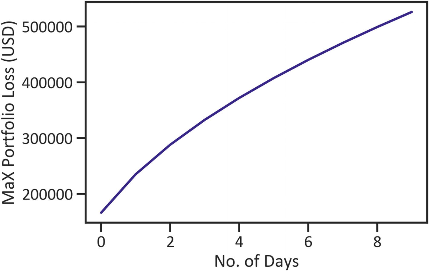
Max portfolio loss (VAR) over a 15-day period
Figure 7-2 shows that as we increase the number of days, the maximum investment portfolio increases too. In the next section, we explored Monte Carlo simulation.
Understanding Monte Carlo
Monte Carlo simulation uses resampling techniques to combat sequential problems. It reconstructs real-life conditions to identify and understand the results of the preceding occurrences and predict future occurrences. It also enables us to experiment with different investment strategies. Not only that, but it performs repetitive measurements on random variables that come from a normal distribution to determine the probability of each output, and then it assigns a confidence interval output.
Application of Monte Carlo Simulation in Finance
Scraped Data
Dataset
Date | High | Low | Open | Close | Volume | Adj Close | return |
|---|---|---|---|---|---|---|---|
2010-11-01 | 58.257679 | 56.974709 | 57.245762 | 57.381287 | 1736400.0 | 46.094521 | 0.000000 |
2010-11-02 | 58.438381 | 57.833035 | 57.833035 | 58.357063 | 1724000.0 | 46.878361 | 0.017005 |
2010-11-03 | 58.501625 | 57.354179 | 58.221539 | 58.076981 | 1598400.0 | 46.653362 | -0.004800 |
2010-11-04 | 59.143108 | 58.140224 | 58.483555 | 58.971443 | 2213600.0 | 47.371891 | 0.015401 |
2010-11-05 | 59.260567 | 58.826885 | 58.926270 | 59.034691 | 1043900.0 | 47.422695 | 0.001072 |
Run Monte Carlo Simulation
Run the Monte Carlo Simulation
Plot Simulations
Simulations
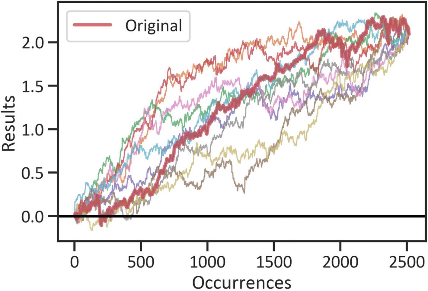
Monte Carlo simulations
Raw Simulations
Raw Simulations
Original | 1 | 2 | 3 | 4 | 5 | 6 | 7 | 8 | 9 | |
|---|---|---|---|---|---|---|---|---|---|---|
0 | 0.000000 | -0.018168 | -0.002659 | -0.021098 | -0.006357 | 0.018090 | -0.010110 | -0.006555 | -0.004119 | 0.020557 |
1 | 0.017005 | 0.005521 | -0.014646 | 0.000541 | -0.009134 | -0.000602 | -0.006801 | -0.003373 | 0.004342 | -0.002257 |
2 | -0.004800 | -0.003900 | -0.002494 | 0.027738 | 0.005924 | -0.012834 | -0.004095 | -0.003315 | 0.000116 | 0.113851 |
3 | 0.015401 | 0.006688 | 0.001144 | 0.005586 | -0.004924 | 0.011399 | 0.009817 | -0.001273 | 0.006164 | 0.023355 |
4 | 0.001072 | 0.005617 | 0.010052 | 0.011748 | 0.007878 | 0.010080 | -0.008666 | -0.005126 | 0.036459 | 0.015438 |
Monte Carlo Statistics
Monte Carlo Statistics
min | max | mean | median | std | maxdd | bust | goal | |
|---|---|---|---|---|---|---|---|---|
s | 2.094128 | 2.094128 | 2.094128 | 2.094128 | 2.145155e-15 | -0.164648 | 0.2 | 0.8 |
Table 7-6 highlights the dispersion. It also highlights the maximum drawdown (the maximum amount of loss from a peak).
Conclusions
When investing in a stock or a set of stocks, it is important to understand, quantify, and mitigate the underlying risk in an investment portfolio. This chapter discussed VAR; thereafter, it showed ways to calculate the VAR of an investment portfolio, followed by simulating stock market changes by applying Monte Carlo simulation. The simulation technique has many applications; we can also use it for asset price structuring, etc. The next chapter further expands on the investment portfolio and risk analysis.