Red invariant : No red node can have a red parent.
Black invariant : All paths from a node to any of its leaves must traverse the same number of black nodes.
These two invariants guarantee that the tree will be balanced. If we ignore the red nodes, the black invariant says that all paths from the root to a leaf have the same number of nodes, which means that the tree is perfectly balanced. The red invariant says that the longest path cannot get arbitrarily longer than the shortest path because it can have a maximum of twice as many nodes—the red nodes that we can legally add to a path of black nodes.
For practical purposes, we will give all empty trees the same color. If we use None to indicate an empty tree, then we are forced to define a color for it, since we cannot add attributes to None, but even if we use our own class for empty trees, there are benefits to defining the color of an empty tree rather than having an explicit attribute. If we do this, then we have to define the color of empty trees to be black.
Exercise: Try drawing a search tree that holds two values, that is, has two non-empty trees, where one has two empty children and the other one empty child. Try coloring the empty trees red. Can you color the non-empty nodes so the tree satisfies the two color invariants? What if you color the empty trees black?
When we search in a red-black search tree, we use the functions we saw in the previous chapter. A red-black search tree is just a search tree unless we worry about balancing it. We only do that when we insert or delete elements, and this chapter is about how to ensure the invariants are upheld at the end of the two operations that modify the tree.
A Persistent Recursive Solution
Our first solution will be a persistent data structure, where we build new trees when we perform the operations. It will then, naturally, be based on recursive functions. We move down the tree to insert or delete as we did in the persistent solution for the plain search trees, but this time we will restructure the tree when we return from recursive calls. Whenever we recognize that the invariant is violated, we transform the current tree to satisfy the invariant.
Insertion
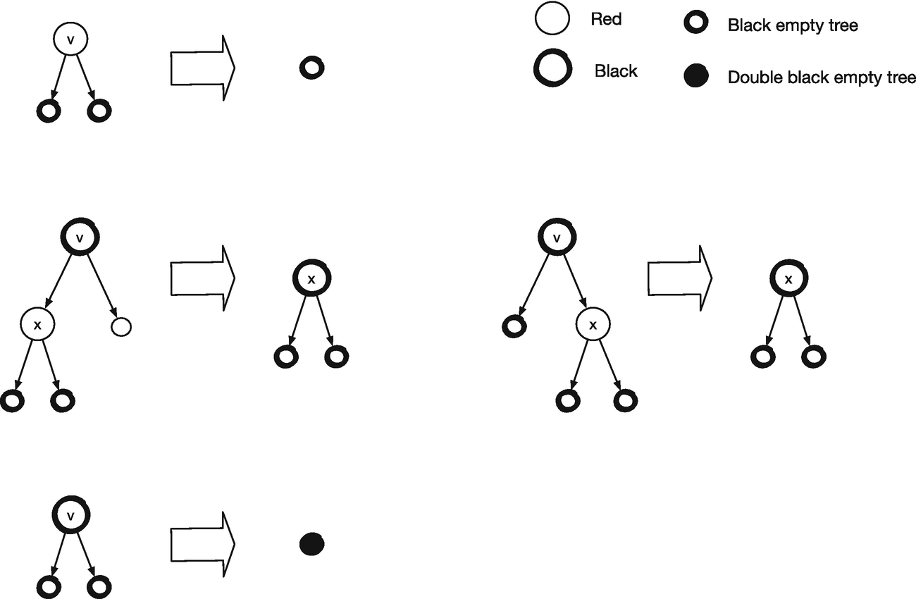
Insertion is the easiest, so let’s handle that first. As earlier, we search down until we find the place where we should add the new node. The empty tree that it will replace is, by definition, black, and its children will also be black. If we color it black, its children will be one black node lower than the leaf we replaced, which breaks the invariant. So we color it red. Now the first invariant is satisfied, but we have violated the second if the new node’s parent is red. As we return from the recursions, we will get rid of red nodes that are the parent of a red node by rearranging the tree. Unless we add extra red nodes when we return, which we won’t, there will at most be one such case, so we only need to check for that. The transition rules in Figure 15-1 will restructure trees that violate the red invariant. If you have any of the trees around the edges, you need to translate it into the tree in the middle.
All the trees a, b, c, and d satisfy both the red and black invariants because the tree as a whole satisfies the black invariant, and the only violation of the red invariant is the two red nodes we see in the figure. When we transform the tree, the number of black nodes down to the leaves in a, b, c, and d remains the same. We remove one above them and replace it with another; we have two new black nodes, but not on the same path. It doesn’t matter if any of a, b, c, and d have a red root because their root’s parent is black in the transformed tree. I will leave it to you to check that the order of the trees is preserved. After the transformation, we have gotten rid of the two red nodes in a row, but we have created a tree with a red root, and if its parent is red, when we return from the recursive call, then we see one of the cases we must handle again. Not a problem, though; we do the transformation all the way up to the root. We might still have two red nodes in a row at the root—the transformations are only applied for trees with black roots. If we end up with two red nodes there, we need to fix it to still uphold the invariant. But that is easy: just color the root black every time you return from an insertion. Coloring a red root black adds one black node to all the paths, but since it is to all the paths, the invariant is satisfied.

Balancing rules for inserting in a red-black search tree
I have split the insertion function from the previous chapter into two to set the root’s color to black at the end. We have an assignment to an attribute there, so it might look like we are modifying the data structure and not getting a persistent one, but it will be a new node that doesn’t interfere with previous references to the set.
For balance() , you need to check if the tree it takes as input matches any of the four cases and then return the updated tree. Otherwise, it returns the input tree unchanged. The checking part , though, can be unpleasant to implement. You could check that “Is this node black, and does it have a left subtree with a red node, and does that subtree have a right subtree that is also red? And if so, extract x, y, z, and a, b, c, and d.” And you have to do that for all four trees. Chances are that you will get at least one of the tests wrong or extract the wrong tree in one or two cases. I don’t know about you, but I don’t want to write code like that. I want to tell Python which tree should be translated to which tree and then have it figure out how to test if the tree matches the from topology and, if so, create a tree that matches the “to” topology. And because I want to solve the problem that way, you now have to learn about domain-specific languages (DSLs).1
A Domain-Specific Language for Tree Transformations
A domain-specific language, or DSL, is a programming language that you build for a specific task. Python is general purpose because you can use it to write any kind of program, but domain-specific languages are usually much more restricted. In my opinion, they are underappreciated and should be used much more. You pay a small price upfront by implementing the code necessary to process it, but it pays off quickly when you avoid writing repetitive, tedious, and error-prone code. And I hope that the following two examples of how we can implement a DSL for our tree transformations will show you that it is not something to fear.
We use exactly the same Node class , but we use strings for the values and the subtrees that aren’t part of the pattern, that is, a, b, c, and d.
It is a recursion on both pattern and tree, where we extract a subtree if the pattern is a string—in our case, that would be when we have “a,” “b,” “c,” or “d.” If we hit a leaf, None, before we expect it, we can’t match and throw an exception (that we have to catch in the balance() function). If the colors don’t match, we also raise the exception. Otherwise, we get the value in the tree and continue matching recursively on both subtrees.
You might now think that this was more complicated than simply implementing the four transformations yourself, and perhaps it is. Still, it didn’t take me much longer to write the automatic transformation than it would take me to implement one or two of them manually, and I only have one function to debug if something went wrong. And if you need more transformations—and you will—then the DSL pays off even more.
I am not quite satisfied with this solution, however, so I will show you another. The implementation we just made is something you can do in all programming languages; it doesn’t involve particularly high-level features. However, we have to parse the DSL each time we try to match a tree, which takes time, and for an efficient implementation of a search tree that might make many insertions, we should want to save as much running time as we can. I also don’t like that we have the patterns inside the balance() function . It makes the function look more complex than it really is. We could put them outside in a list, of course, but if we later add more from and to patterns, we must be careful to match them up correctly. So I want to do something else that is more to my liking.
The next solution, which is more efficient and more aesthetically pleasing, requires that we create functions on the fly. Some languages have better support for this than Python, and some have no support for it at all. There are always ways to do it, but it can be hard. It is not in Python, though.
We will create functions for matching a pattern and returning a transformed tree (or raise an exception if we can’t). We generate the functions’ source code from the “from” and “to” tree specification and ask Python to evaluate the source code and give us the function back, and that will work just as well as if we had written the functions ourselves.
This is the rule for the leftmost tree, and you can check it if you want. We don’t explicitly check for whether a subtree exists; we just extract trees and hope for the best. In some languages, that could crash your program, but in Python, we will get an AttributeError if we try to get an attribute out of None, and then we just change it into a MatchError.
We have two helper functions, one for generating the lines inside the try block, collect_extraction(), and one for generating the output tree, output_string(). We get to them in the following. We wrap them in the function definition, func, that defines a function named rule, putting the subtrees and value extraction code in the try block followed by the returned tree, which is created if the extraction code doesn’t fail, that is, if we match. The exec() function is where the magic happens. It will evaluate the code we give as the first argument in the namespace we give as the second argument. We give it globals(), which is the global scope. That is where it can find the Node() class that it needs for the return value. The last argument is a dictionary where it will put the variables we define. We define one, rule, that we extract and return.
We give it a node in the pattern structure as the first argument, a variable where we can extract values from, and the list it should put the code into. We return the list at the end to make it easier to get it in the transformation_rule() function . The idea is that we name all the subtrees of a node, so we can use the name to extract nested information. When we call it the first time, in the function we create, the node is tree, and we will assign tree to a variable that is the same as the value in the pattern. If that is all there is, we are done here. We have assigned to the variable the value we want it to have. However, if it is a node, we recurse on the subtrees and tell them that they should get values from the left and right subtrees. When we have recursed, we change the variable to its value because it is the value we want in the output tree.
Adding more transformations later is also more straightforward now. We have to create a rule function for them, but our process for doing that can handle any transformation, so they are easy to add. We might have spent a little more time developing the DSL, but it will soon pay off because now we need to implement deletion, and there we have to add more rules.
There is another issue, though, that we might as well deal with. There are symmetries in the trees—the left and the right are simply mirrored vertically, as are the top and bottom trees (if you ignore the names we give the nodes and the subtrees). If we hand-code the pattern matching, we have to deal with all four cases, but with our DSL, we can write a function that mirrors the trees and use those. The fewer transitions we have to explicitly implement, the better, and that includes specifying them in the DSL. It is tedious, and it is error-prone, so writing symmetric cases is something we would like to avoid if we can, which of course we can. The computer is good at doing simple things like mirroring a tree—we just need to mirror a node’s children and then switch left and right. For the transformations, we need to mirror the “to” tree as well for this strategy to work, since otherwise, we put the values and subtrees in the wrong order; I will leave it as an exercise for the eager student.
Exercise: Convince yourself that you get the same transition for the right rule if you flip both left and middle trees and that you get the same rule for the bottom tree if you mirror the top tree and the middle tree.
Of course, it didn’t save us any work this time because we had already implemented all four rules, so if this is all we had to do, there wouldn’t be much point in coming up with the smarter solution now. That is something we should have thought about before, but now it is too late. If we need to add more transitions, however, it could come in handy.
Deletion
Deleting leaves in red-black search trees
Cases for parent nodes of double black nodes
But can I ignore the empty subtree cases in my code? Yes, if I redefine what it means for a tree to be empty, I can. I will use actual nodes as empty trees and say that a tree is empty if both its subtrees are None. I won’t allow a tree with one None tree and not the other, but there is nothing wrong with representing empty trees by special variants of nodes. It is merely another way to introduce a dummy element to simplify our code.
With this class, and by considering empty trees those with None subtrees , I can pattern match subtrees of an empty tree. As long as those subtrees go back into the same node, I can replace the color of a leaf during a pattern match transformation rule. I will get into trouble if I create a node that isn’t empty but has a None child, but I check if that happens in the constructor and throw an exception if it does. None of the rules we will apply will do this. You could argue that since I only check the subtrees in the constructor, nothing prevents us from explicitly setting a subtree to None , and that is correct. In the persistent version of red-black search trees that we are currently implementing, that doesn’t happen, though. We never change a node once it is created.
It would be great if we could use EmptyTree as default parameters for the Node constructor, but this isn’t possible. We cannot create EmptyTree before we have defined Node, and by then, it is impossible to set the default parameters. (Well, there are hacks, trust me, but I don’t want to go there.)
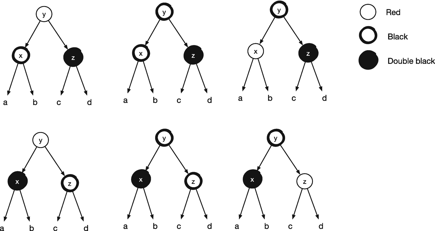
Now consider the cases in turn, starting with the two that have a red root. In these cases, we can move the black node to the top. We keep one of its children, whose subtree must satisfy the invariants as it hasn’t changed in the removal (that change must have happened in the subtree with the double black node). We keep it under a black root, so we don’t introduce a violation of the red rule, and since it has as many black nodes above it as before, the black invariant is also preserved. We put the other child under the red node. It doesn’t add or remove any black nodes on the path to the root, so the black invariant is preserved. The red invariant might now be violated, so we need to balance the tree—we get there in a second. For the double black tree, we can change it to black. We have added a black node above it, and that compensates for the black node missing in a double black node. You can see the transformations at the top row of Figure 15-4. We keep the subtrees of the double black node in the same tree: a and b stay under x on the left; c and d stay under z on the right. That means that even if the black node was empty and those trees were None, we wouldn’t risk moving None into a node higher in the tree. If the double black tree is empty, then the new black tree is empty as well, but we don’t create a new tree that would invalidate our rule about None subtrees.

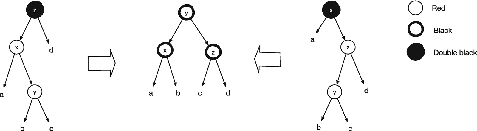
Rotation rules for removal
If we have a black root and a red subtree, we cannot transform the tree using just that. You can try out the different transformations, and you will find that they do not work. We can, however, look a little bit further down the red subtree. A red subtree will have black children because of the red invariant (and because empty trees are black or double black, so red trees must have subtrees). If we count the number of black nodes in these trees, we must also conclude that the children of the red node are not empty. There are at least three black nodes on the path from the root to the children of the double black node, one for the root and two for the double black. Therefore, there must also be at least three black nodes from the root, through the red node, down to the leaves. If any of the red nodes’ children were empty, then there would only be two black nodes from the root to a leaf, so they cannot be. That means that it is safe to move the subtrees of the red node’s children around. The double black tree might be empty, so its children might be None, but we keep them together in the transformation, so we won’t have problems there either. To see that the transformation will preserve the black invariant, you simply have to count how many black nodes you get down to the subtrees a–e. I will leave that as an exercise for you. After we perform the transformation, we might have violated the red invariant. We put a red node about the c tree on the left, and c might have a red node as it had a black parent before. On the right, we put a red node above the c tree as well, and the same argument goes—we might have put a red node on top of a red node. Thus, again, we have to balance the tree afterward.
These transformations, which we will call rotations , eliminate the double black node or move it up toward the root where we can get rid of it. They all satisfy the black invariant, but all of them can violate the red invariant. The top row can be handled by the balancing rules we had for insertion. They handle all cases where we have a black root and two red nodes following it down a path. The rules cannot handle the second row. They do not know how to handle a double black root. No worries, there are two cases where we can have a double black root and two red nodes in a row, and we can rebalance them easily; see Figure 15-5.
For the last row, we can apply the insertion balancing rules again; we just need to do it for a subtree of the root, y on the left and z on the right. Those are the trees with a black root where there might be two red nodes on a row.
Double black balancing rules
There, we need to call balance() on a subtree of the transformation and not the full tree. We could implement the rotations using transformation_rule() as for the balance() function and then call balance() after rotation transformations, but that isn’t good enough for the last two rules. There we need to call balance() as part of the transformation. And our DSL cannot handle that.
This happens all the time. You write a DSL or a function or a class that handles the cases you have seen so far, and then something appears that goes beyond the rules you thought were all there was to it. Not to worry, though, it is usually a simple matter of fixing it. Not always, sometimes your original thinking is fundamentally flawed, and this becomes apparent when you run into new cases, but usually, you can extend or generalize your code a little to handle new cases.
It might be overkill to add two classes just to add balancing to transformation patterns, but it isn’t complicated code, and it makes the expressions easy to read. So if I need to call functions in many patterns, the work will pay off quickly.
Here we create a new Function object with the function name from the tree FunctionCall object and call it to build a new FunctionCall object . Don’t modify tree.expr, which would be the easy solution because the same object sitting in the un-mirrored pattern would be affected.
For the rotation rules, I will put Balance() around the output specification for the first two rows, so balance is called there, and for the last row, I will put Balance() on the appropriate subtree.
Pattern Matching in Python
The DSL we wrote for transforming trees is based on matching a pattern of trees and then transforming the tree. This kind of pattern matching is built into some programming languages, but at the time I am writing this, it isn’t yet in Python. It is being added, however, so by the time you read this, it might already be there. When it is already in the language, we don’t need to implement it ourselves.
I cannot promise that it will look exactly like the following code, but the current beta releases of Python look like what I will show you. To match a pattern, you use the match keyword , and after that you have a list of patterns to match.
The top four lines in the class definition tell Python which variables we can match against and what type they have. The __match_args__ specifies the order the variables will come in. If you leave it out, you can still pattern match, but then you must use named variables in the matching.
As you can see, it is close to the DSL we wrote (which isn’t a coincidence), but now directly supported by the Python language.
Useful domain-specific languages often make their way into languages like this, and when you are reading this book, you might already have this kind of pattern matching in Python. It is still useful to know how to implement your own little languages, however. Not all such languages get promoted into the main language, and when you need one, you can’t wait the years it takes before they do. So don’t feel that you wasted your time on that part of this section.
An Iterative Solution
The persistent structure is sufficiently fast for most usage, and since we balance our trees to logarithmic height, we are unlikely to exhaust the call stack in the operations. However, we can get a little more speed with an iterative solution, where we save the overhead from function calls, and that solution also eliminates any call stack worries.
If the DSL, and the tree transformations with it, seemed overly complicated, then I have good news. The iterative and ephemeral solution is simpler if we implement it the right way, but we need to take a detour through more complicated rules. With the new solution, we will look upward in the tree instead of downward. It reduces the number of cases we need to consider substantially. A node only has one parent, one sibling, one grandparent, one uncle (parent’s sibling), and such. In the previous section’s insertion rules, we had four cases, but if we look from the perspective of the lower red node, we can match all of them simply by checking if it has a red parent. With the right abstractions added to nodes for examining the tree structure, we will eliminate all symmetric cases and simplify the pattern marching. We couldn’t easily do the same thing with the persistent solution since we constructed new trees in recursion, but when we allow ourselves to move around a tree and modify it, we have more options.
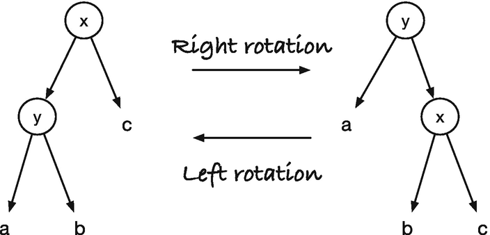
Left and right rotations
We won’t use exactly the same transformation rules as with the persistent structure. There, we need to continue building a new tree all the way up from the recursion, but now we can restore the invariants early and terminate. Tweaking the rules a little, by examining slightly more of the tree, we finish processing with a constant number of tree rotations per insertion and deletion and an amortized constant number of color changes. But before we get to that, we must add the necessary functionality to nodes.
We first need to update our Node class . In the iterative solution, we need to run from leaves toward the root when we balance a tree, so we need to add a parent pointer. We will use the WeakRefProperty class from Chapter 10 for the parent reference, so the reference counter garbage collection will work. To ensure that children and parent pointers are always consistent, we can add getters and setters and put them in property classes . If we set a child of a node, we make sure that its parent is set accordingly. We will use a dummy class for empty trees, so we won’t worry about not setting the parent of empty trees. We use the same object for all empty trees, so an empty tree’s parent will be the most recent node we added it to, but we only use the parent reference of an empty tree in one place, which is when we delete, and there it will point to the correct node (because we set it to point there just before we use it). The other reason we use a dummy node for empty trees is that we want to be able to check the color of empty trees, find their siblings and similar, and check if in all ways they behave like trees, but just not hold any data or subtrees.
Instead of putting a color in the empty tree, I chose to use is_red and is_black properties . I just find that this makes the code more readable, but it is a matter of taste. The @property decorator creates a property object (it calls the property constructor the way all decorators do). When used this way, we only give it a getter method—when we have used it earlier, we have called the constructor more explicitly and provided both a getter and a setter. When we use it as a decorator, we implicitly call the constructor with a single argument, the method we define following the decorator, so we give it a getter. For these properties, getters are all we need.
These properties give us a language to query a tree’s structure, and you can consider it a new domain-specific language if you like. It has the qualities of one. We just usually do not call it that if we are simply using the features that Python readily provide us with.
It is not pretty, but it gets the job done and allows us to make the basis of the recursive type definition an instance of the type itself.
Checking if a Value Is in the Search Tree
Inserting
To fix the red invariant, we use these alternative rules that let us limit the modifications to the tree structure to a maximum of two and have all remaining updates simply change colors. Since modifying the tree structure is more expensive than changing colors—you have to update references to other nodes and not just a single value—there can be speedups in that. The rules are shown in Figure 15-7, except for symmetric cases. The arrow points to the node we are carrying in fix_red_red() . If you are in Case 3, you have restored the red invariant after the transformation. If you are in Case 2, you will be in Case 3 next, and only in Case 1 can you continue iterating; see Figure 15-8 where Start is where we consider which tree to transform, the arrows are how the transitions can be chained together, and Done is when we stop rebalancing the tree.
Case 2 and Case 3 change the tree structure, but you can only be in these cases twice per insertion (once for each). Case 1 only changes colors. With these rules, then, we always have a constant number of transformations. We shall see later that we also have an amortized constant number of color changes. Insertion still takes logarithmic time—finding where to insert a value costs a logarithmic-time search—but maintaining the balancing invariants is only constant time on top of that.

Alternative rules for correcting the tree after inserting

Transitions between cases when inserting
I think you will agree that even without a DSL, this version of the data structure is simpler to implement. Removing the symmetries by looking up in the tree dramatically simplifies things.
Deleting
The core idea for deletion is the same as always. Find the node to delete, and if it has two children, get the rightmost value in the left subtree, put it in the node, and delete the rightmost value from the left tree. If we need to delete a node with at most one subtree, then we get the non-empty subtree (or an empty one if they are both empty) and replace the node we delete with this subtree. If the node we delete is red, then we can’t have violated any invariant. Both parent and child must be black, which means that we add a black node to a black node to not violate the red invariant. A red node doesn’t count toward the black depth of paths, so removing it doesn’t change anything, and thus the black invariant is satisfied. If the node we remove is black, however, we might be in trouble. The replacement might be red, in which case we risk invalidating the red invariant. That is an easy fix. We can color it black, and then the red invariant must be satisfied. If it was originally red, painting it black would satisfy the black invariant as well—we replaced its black parent with it, removing one black node from the paths, but then we added one back when we painted the replacement black. If it was already black and we paint it black again, we have painted it double black, and that is something we must fix.
We don’t color any nodes extra black, but we use the color as a conceptual color representing an extra black node on paths down to leaves in a subtree as we did in the persistent solution. There, we needed the extra color for pattern matching, but now we will start each transformation with a reference to the one node that is double black, and that gives us all the information that we need about it.
There are many trees we could potentially have to match for transformations, depending on whether we have empty trees or such (although having dummy nodes for empty trees helps a lot). However, we can make an observation that limits the numbers somewhat. If we consider the double black node and its sibling, we will find that the sibling always has two non-empty trees. The path from the rule to a leaf in the subtree under the double black node is one black node short of the paths that go to leaves in the sibling’s subtree, and the double black node is black. If the sibling is black, then black paths in the subtrees must count to the same as the subtree under the double black node, and it has at least a length of two (itself and its empty children, if they are empty). Therefore, the sibling’s children must have (possibly empty) subtrees. If the sibling is red, you can run the same argument, except that the children must be larger still. This means that we can always assume that the sibling has non-empty children and consider trees consisting of the double back node, its parent, its sibling, and its sibling’s children.
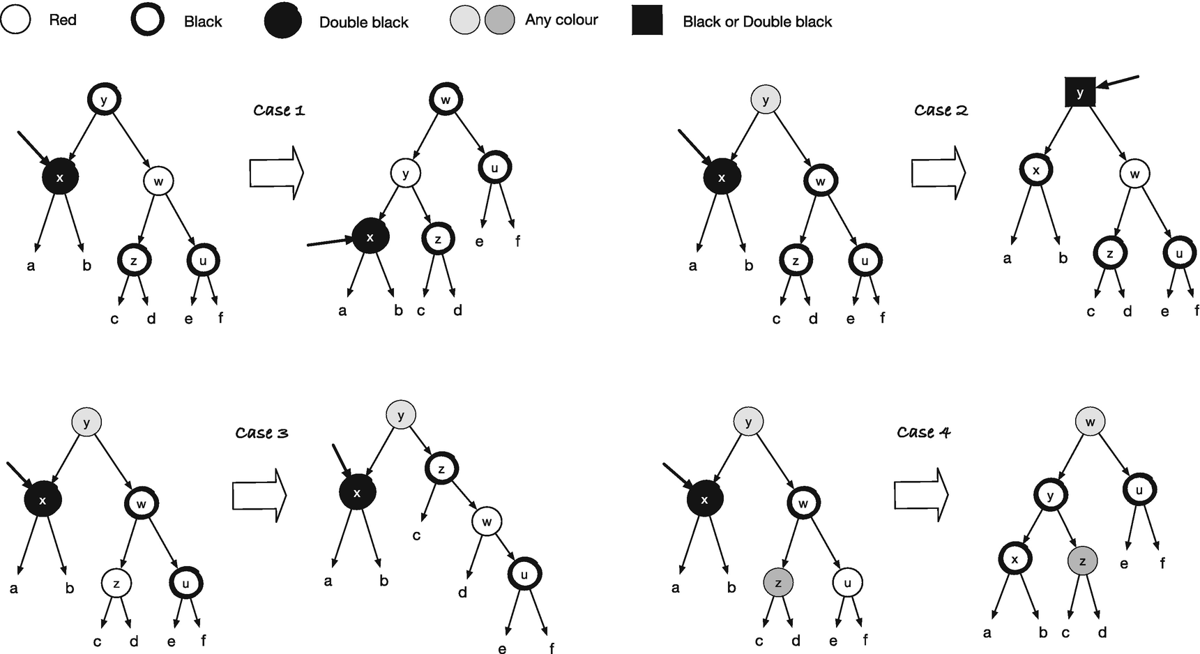
We consider all combinations of the double black node, its parent, its sibling, and the sibling’s children for the new rules. That means all combinations of colors that satisfy the red invariant (i.e., if the parent is red, then the sibling cannot be red as well and such). I count the combinations to 18 (but I might be wrong, so you better check me). Luckily, we can cut it in half by considering symmetries, and it turns out that some of the rules are indifferent to some of the colors. You can see the new transformation rules in Figure 15-9 for the cases where the double black node is a left child. The four cases where it is a right tree are symmetric, and we can get them using the mirror() function.
Exercise: Convince yourself that these rules, combined with their mirrors, cover all combinations of a double black node, its parent, its sibling, and its sibling’s children.
The gray nodes are either red or black, and except for Case 2, they retain their colors in the transformation. In Case 2, the root will be painted either black or double black by the transformation: black if y is originally red and double black otherwise (think of it as painting the node black, but when you paint a black node black, it becomes double black).
Rotation rules for iterative deletion
Transitions between cases when deleting nodes
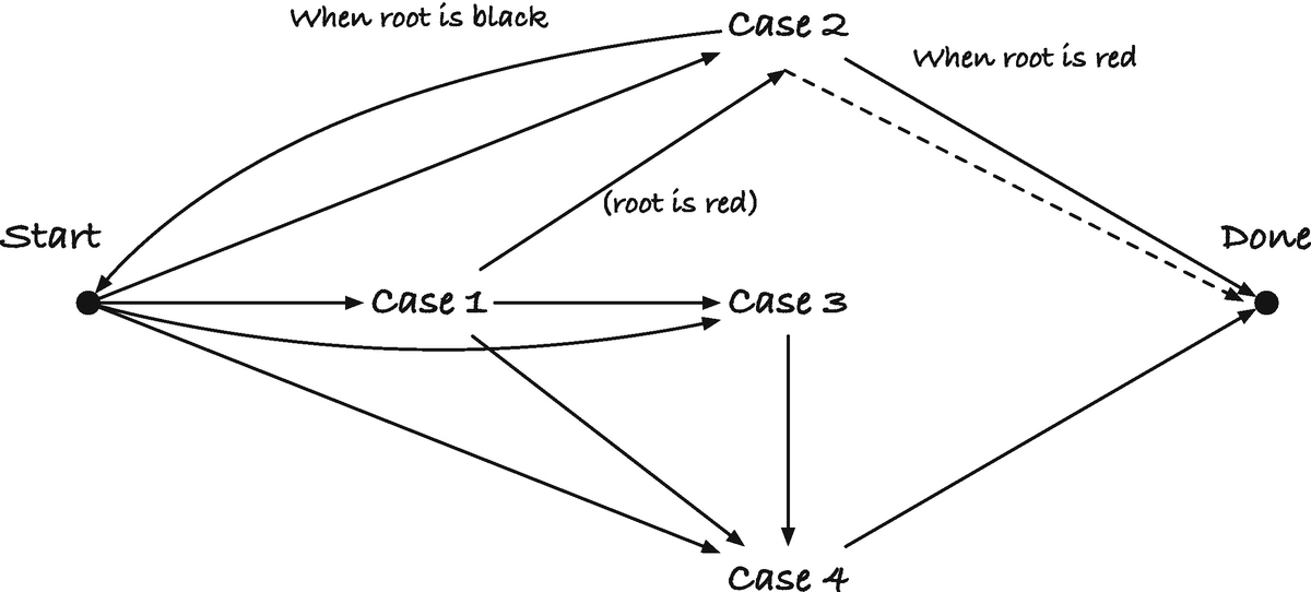
Notice that since it is only possible to visit Case 2 more than once, we can’t change the tree topology more than three times (the longest such path is Case 1 to Case 3 to Case 4), after which we only change the color of nodes. With a more elaborate DSL (as I hinted at when we discussed insertions), you can optimize the code and only update the attributes you strictly need. Since updating colors is faster than updating the references when you rotate the trees, it is worthwhile if you need a very fast search tree. Still, it is not necessary for our conceptual understanding, so I will not cover it here. As an exercise for developing a better DSL, however, I think you will find it interesting.
For the black invariant, consider the cases again, and count how many black nodes are above each terminal tree. They must be the same before and after the transformation. In Case 1, there is one black and one double black node above a and b and two black nodes above the others both before and after the transformation. In Case 2, it depends on what color the root on the left has. If it is red, we will color the root on the right black. That adds one black to the tree previously rooted by the double black node, but that simply means that we got our missing black node back, so we can change the double black node to simply black. For the remaining trees, we removed the black on node w but added it to the root, so we end up with the same number of black nodes. With this transformation, if the root on the left is red, we can terminate the fixing run because the double black node is gone. If the input root is black already, we paint the new root double black, leaving the same amount of black for a and b, but we have removed one black for the other trees, replacing it with a double black. This means that they have one black less than before (because double black means that we are lacking one black), but with the double black at the root, that matches the count. For Case 3, there is one double black above a and b before and after the transformation, one black above c and d before and after, and two black nodes above the remaining two trees, both before and after the transformation. Finally, for Case 4, we have a double black node above a and b. We change that to two black nodes, settling the accounting of the missing black. For the remaining trees, we have the same number of black nodes before and after the transformation.
I chose to match against the cases in a different order than in the figure since I found it easier to determine which case we are in using this order—where we can use the information we get from one test in the following—but otherwise, it is a simple translation of the transitions in the figure. However, there is one issue that the figure doesn’t show but which we must handle in the implementation. The node we are working on can be the empty tree, and there is only one empty tree. That means that if a rotation involves an empty tree, then its parent will have changed. Therefore, I get the parent of the node before transitions and set it again after rotations, so we can continue the rebalancing after handling each case. You could get out of this problem by having separate empty trees every time you need one, but that would double the tree’s space complexity.
Resetting the parent reference a few times in a single function is a small price to pay for not spending twice the memory we need.
That is all there was to removing elements.
The Final Set Class
An Amortized Analysis
When we insert and delete, we spend O(log n) time, but we can split this time into the part that involves finding the location where we need to insert a node or delete it, which is the logarithmic-time search in the tree, and the time we spend on restoring the red-black invariants. If the tree is balanced, we cannot do better than logarithmic time for finding the location, but perhaps we spend less time than that on fixing the tree afterward. With a detailed analysis of the operations, we can show that we do indeed spend less time; we spend amortized constant time restoring the invariants, provided we use the rules in Figures 15-7 and 15-9.
The argument is slightly more involved than those we have seen earlier and requires a potential function. The idea here is to assign a potential to the current state of a tree so that the potential can never become negative. With each operation, we count how much the potential changes. If we cannot increase the potential by more than a fixed amount over all the operations we perform, then we cannot decrease it more than that either, since it cannot get negative, so once we have the function, the goal is to see that the increases are limited.
We will assign a potential to a black node: a black node with one red and one black child has a potential of 0, a black node with two black children has a potential of +1, and a black node with two red nodes has a potential of +2. All transformations we only perform once per operation can only add a constant amount of potential, limiting the increase of the potential to O(n) from these operations. What we need to examine in detail are the transformations we can do more than once per insertion and deletion, and we need to show that for those, the potential decreases. Those transformations are Case 1 for insertions and Case 2 for deletions.
Consider Case 1 in the insertion transformations. The z node has a potential of +2 because it is black with two red children. Nodes y and w have a potential of 0 since they are red nodes. The children of w must be black since it is red, and we have to keep that in mind when we change it. We do not modify the other terminal nodes’ colors, so we cannot change any potential there. When we color z red and its children back, we remove -2 potential. When we color w black, we add +1—it is red, so its children must be black—which gives us a total reduction of -1 when applying the case. When the potential is decreasing, we cannot run it more times than we have added potential, which is O(n) for n operations, provided that the deletion case doesn’t add potential.
Now consider Case 2 for deletions, and assume that y is black. If it isn’t, we terminate the update, so that rule can only run once per deletion and thus can only add a constant amount of potential per deletion. We have a potential of +1 in y because it has two black rules, and we have a potential of +1 in w for the same reason. When we color w red, we remove -1 potential from y and -1 from w, so doing the transformation decreases the potential by -2.
We conclude that we have a constant number of tree transformations for both insertions and deletions, a maximum of two for insertions and three for deletion, and a number of color changes that are amortized constant. Rebalancing is thus fast; we do not pay much of an overhead compared to a normal search tree. We get a balanced tree that can at most have a factor two difference in paths to a leaf, so compared to perfectly balanced trees, with high log2 n, we can spend 2 log2 n on all operations where we need to search in the tree. So we can say that we get within a factor two of a perfect search tree for a constant amount of work.