Chapter 12
System Design Foundations
Once you have decided on the attributes you want to quantify and the scale of numbers you would like to use, it's time to look at more factors in creating a mass amount of data objects. In the next steps, you learn how attributes of different quality get different numbers and how to properly name all the data objects you create.
After you have assigned numbers to every attribute, it is a good idea to add them all up so you can compare the different data objects against each other. By getting a total score, you can start to get some insights into the balance of all the data objects in comparison with each other.
Attribute Weights
This section shows how to find attribute weights for the racing example from Chapter 11, “Attribute Numbers.” Table 12.1 shows how you would get a total score for each car, based on its attributes (refer to Table 11.1).
Table 12.1 Adding the attributes for each car
Car |
Acceleration |
Top Speed |
Total Value |
|---|---|---|---|
Sports car |
8 |
8 |
16 |
Muscle car |
6 |
10 |
16 |
Motorcycle |
10 |
6 |
16 |
Now, you need to test these numbers in a game. For this example, you would race all three cars several times and find out which one wins most often and by what margin. Let’s say that in this testing, the muscle car wins every race by a significant margin. You are now seemingly stuck: The data is clearly not balanced if one car is winning every time. But if you lower either attribute value for the muscle car, its total won’t be as high as the totals for the other two cars, so you will no longer be able to compare them in the spreadsheet.
This kind of situation happens with game data all the time. It’s actually fairly rare for attributes to add up across balanced game objects to be the same. It often turns out that one attribute is simply more important in the context of the game than others are. In the case of our racing example, the more important attribute appears to be top speed.
If we add one more attribute to our cars, we can get an even better idea of how badly skewed raw attribute numbers can be. Table 12.2 shows an additional attribute, horn sound, and one more car.
Table 12.2 An additional car and an additional attribute
Car |
Acceleration |
Top Speed |
Horn Sound |
Total Value |
|---|---|---|---|---|
Sports car |
8 |
8 |
4 |
20 |
Muscle car |
6 |
10 |
4 |
20 |
Motorcycle |
10 |
6 |
4 |
20 |
Clunker |
1 |
1 |
30 |
32 |
If you simply look at the total raw scores for the car, it seems like the clunker is far and away the best vehicle. However, when you look at the attributes in the context of what they do in the game, you see a very different picture. This is a racing game, so the loudness of the horn is not important to the game, even if it is an attribute you can control. The problem is that attribute value is throwing off the total value of each car.
The solution to this problem is to use attribute weights. An attribute weight is a multiplier you apply to each attribute that compensates for some attributes being more important than others. When setting up the data at first, using 1.0 is a nice neutral starting point. It indicates that all attributes are equally important and lets you get through the data entry process more quickly. When you begin testing, you are likely to find that the attributes are not of equal value, and they need to be modified with weights. In the racing example, testing shows you that top speed is more important than acceleration, and horn loudness is not very important at all. You can use these observations to inform your first pass with weights, which might look something like this:
Acceleration: 1.0 (Neutral. Not very important but not unimportant.)
Top speed: 1.5 (Top speed is therefore 150% as important as acceleration.)
Horn sound: 0.0 (This essentially removes horn sound from the total value equation since it is not an important factor for the game.)
You can now recalculate the weighted total for each car, as shown in Table 12.3.
Table 12.3 Weighted attributes
Car |
Acc |
Speed |
Horn |
Acc |
Speed |
Horn |
Total Value |
|---|---|---|---|---|---|---|---|
Weights |
1.0 |
1.5 |
0.0 |
Weighted |
Weighted |
Weighted |
|
Sports car |
8 |
8 |
4 |
8 |
12 |
0 |
20 |
Muscle car |
6 |
10 |
4 |
6 |
15 |
0 |
21 |
Motorcycle |
10 |
6 |
4 |
10 |
9 |
0 |
19 |
Clunker |
1 |
1 |
30 |
1 |
1.5 |
0 |
1.5 |
With the new weights applied, the total value looks a lot more like the test results you see in the actual game. The muscle car always wins because it has a better total real value in game. The goal of the weights should be to represent the effect of each attribute in the game as realistically as possible.
The next step is to go back to the data and adjust it so that each car has the same total weighted value while retaining its own unique character. Given these goals, you can adjust the attributes on the other vehicles as shown in Table 12.4 to make them feel different from each other, hit your intended goals for the feel of the game, and use balance attribute weights.
Table 12.4 Modified attributes
Car |
Acc |
Speed |
Horn |
Acc |
Speed |
Horn |
Total Value |
|---|---|---|---|---|---|---|---|
Weights |
1.0 |
1.5 |
0.0 |
Weighted |
Weighted |
Weighted |
|
Sports car |
8 |
8 |
4 |
8 |
12 |
0 |
20 |
Muscle car |
5 |
10 |
4 |
5 |
15 |
0 |
20 |
Motorcycle |
11 |
6 |
4 |
11 |
9 |
0 |
20 |
Clunker |
1 |
1 |
30 |
1 |
1.5 |
0 |
1.5 |
With these new numbers, it appears as though you have reached all your goals—but there is only one way to find out. After doing a balancing pass with weights, you need to go back and test the feel of the game. If the game now feels more balanced, you can conduct some specific tests to find out how many times each car wins and by what margin. When you have that information, you can be more confident that your game is more balanced, and you will be able to add new objects to your spreadsheet and quickly get them into balance before ever actually placing them in the game.
One more factor we need to look at here is that the clunker is still way out of balance. This type of imbalance is not always a bad thing or something that needs to be fixed. This might be a joke car that was placed in the game, or it could be a punishment for a player who wrecks a car too often that will set up the player for almost certain failure. It could even be a challenge car that a very good player might pick to show that, even with the quantifiably worst vehicle in the game, they can still win. These are just some of the valid reasons to have data objects that are well out of balance. It is just as important that you know they are out of balance and by how much.
It is important to note that weighting can require some counterintuitive thought. In Table 12.4, you can see that speed is weighted 1.5 and acceleration is weighted 1.0, which means that speed is more important than acceleration in this game. It also means that the raw numbers for speed are likely to be smaller in total than the raw numbers for acceleration.
Let’s consider a more extreme example. Say that you are making an archery game where each archer has the attributes power and accuracy. Because a missed shot does no damage, you have determined that accuracy is twice as valuable as power. In this case, your attributes would get the following weights:
Accuracy: 2.0
Power: 1.0
This means two equal archers would have raw attribute numbers where the power attribute is higher than accuracy in most cases. It’s only once the weight is applied to the raw values that you can see which of the players is the better archer. For example, look at Table 12.5.
Table 12.5 Archer attributes
Archer |
Power |
Accuracy |
|---|---|---|
Archer 1 |
10 |
10 |
Archer 2 |
20 |
5 |
At a glance, if you don’t know the weights, Archer 2, who would have a higher total attribute summed score, looks like the overall better archer. But when you apply the weights, you can see that the two archers are, in fact, balanced (see Table 12.6).
Table 12.6 Weighted archer attributes
Archers |
Power |
Accuracy |
Power |
Speed |
Total Value |
|---|---|---|---|---|---|
Weights |
1.0 |
2.0 |
Weighted |
Weighted |
|
Archer 1 |
10 |
10 |
10 |
20 |
30 |
Archer 2 |
20 |
5 |
20 |
10 |
30 |
Be patient when searching for proper weights. It can take dozens of tests—or more—in varying circumstances with multiple playtesters to determine the proper final weights to apply to your attributes. While this process should start very early in the production of data objects, it’s likely that it will continue throughout production and almost up to the end.
DPS and Intertwined Attributes
Very often, a single attribute tells only part of the story of the in-game interaction. The most common example of this is damage per second (DPS), where a series of characters have both a damage attribute and an attack rate attribute. Each of these has its own scale, with a minimum and a maximum. However, looking at only one part of the pair—that is, looking at only damage or only attack rate—does not explain accurately how powerful the character is. For example, say that you have a pair of weapons—a dagger and a battle axe—which have the damage scores shown in Table 12.7.
Table 12.7 Weapon damage scores
Weapon |
Damage |
|---|---|
Dagger |
6 |
Battle axe |
14 |
Which one of these weapons does more damage? Without any other context, the answer is fairly clearly the battle axe, but let’s look a little deeper. Table 12.8 shows how often each weapon can attack in a minute.
Table 12.8 Weapon damage per minute
Weapon |
Damage |
Attacks per Minute |
|---|---|---|
Dagger |
6 |
17 |
Battle axe |
14 |
7 |
Now which weapon do you think does more damage? While individual hit damage has not changed, the total accumulation of damage output has changed considerably. Instead of asking how much damage each weapon does, it would be more helpful to consider how much damage each weapon does in a single minute. When you take into consideration both the amount of damage done and the frequency at which damage is done, you can get a much clearer idea of which weapon does more damage in a practical setting in the game. Because video game combat goes fast—usually in seconds rather than in minutes—we commonly express this value as DPS (damage per second).
But how do you determine DPS for two weapons that can’t attack every second? To do this, you need to take an intermediate step and calculate using a scale at which both weapons can do damage multiple times. For this example, we can use minutes, but any amount of time will work, as long as it’s enough for both data objects to have multiple attacks. To get the value, you need to multiply the damage of each shot by the frequency:
Weapon damage × Attacks per minute = Damage per minute
Table 12.9 shows the results for the dagger and battle axe example.
Table 12.9 Damage per minute calculation
Weapon |
Damage |
Attacks per Minute |
Damage per Minute |
|---|---|---|---|
Dagger |
6 |
17 |
102 |
Battle axe |
14 |
7 |
98 |
You can now clearly see that the dagger does slightly more damage over time. To translate damage per minute to DPS, you divide the damage per minute value by 60, using this formula:
(Weapon damage × Attacks per minute = Damage per minute)/60
Table 12.10 shows the results for the dagger and battle axe example.
Table 12.10 DPS values
Weapon |
Damage |
Attacks per Minute |
DPS |
|---|---|---|---|
Dagger |
6 |
17 |
1.7 |
Battle axe |
14 |
7 |
1.6 |
With this calculation, you can now compare two weapons meaningfully, and in Table 12.10, you can see that over time the dagger will do slightly more damage than the battle axe. Note that the final DPS value has a decimal portion, so it is likely going to be used only for internal evaluation. If you wanted to represent this to players, it might be better to leave it as damage per minute or show it graphically as a bar chart.
The calculation becomes slightly more complicated when the frequency is measured in delay, as opposed to attacks per time. For example, for the dagger and battle axe, you might have a cooldown delay between attacks. To convert a cooldown into a per time measurement, you divide 60 seconds by the cooldown to determine how many times the cooldown can trigger in a minute. For example, a 3-second cooldown would be 60/3 = 20 attacks per minute.
While DPS is the most common intertwined set of attributes used in games, it’s far from the only one. The good news is that any given set of intertwined attributes can be treated in the same way as DPS for the sake of comparison. Let’s look at one more example that at first seems to be quite different. Say that you have forklifts that can carry pallets. In this game, quickly moving pallets is advantageous, so you want a forklift that can carry a lot of pallets. The other part of the equation is how many trips the forklift can take in a minute. The more trips, the better. Table 12.11 summarizes the capabilities of two forklifts.
Table 12.11 Forklifts
Forklift |
Pallet Capacity |
Trip Duration, in Seconds |
|---|---|---|
Speedy |
5 |
20 |
Big Brutus |
9 |
30 |
Which forklift is the better one in terms of this game mechanic? To compare the two, you need to first calculate how many trips per minute each can make:
Speedy: 60/20 = 3
Big Brutus: 60/30 = 2
These are now your trips per minute scores. Next, you need to multiply the capacity by the trips per minute to get a total pallets per minute score. This gives you a final comparison that looks like what is shown in Table 12.12.
Table 12.12 Compared attributes
Forklift |
Pallet Capacity |
Trip Duration, in Seconds |
Pallets per Minute |
|---|---|---|---|
Speedy |
5 |
20 |
15 |
Big Brutus |
9 |
30 |
18 |
In this case, Big Brutus is the better of the two forklifts over the long run.
When using intertwined attributes, you often use the final DPS comparison score to evaluate weight in the total comparison of data objects instead of the individual attributes.
Binary Searching
Binary searching is a mathematical method of searching that enables someone to find an exact unknown number in the fewest possible guesses. Why is this important to you as a game system designer? You are constantly trying to find the right numbers for your data objects. By using binary searching, you can home in on the number you need more quickly, saving valuable time when creating large amounts of data.
How Binary Searching Works
The way binary searching works is slightly unintuitive, but once you understand how it works, it becomes simple and fast to use. To perform a binary search, you need just a few pieces of information:
Range of viable numbers: For a strict binary search, you need to know the largest and smallest possible numbers that could be correct. There are workarounds for this, as discussed later in this chapter, but they don’t fit the strict definition of binary searching.
Feedback response: This lets you know if your current number is too high or too low. Without knowing this, you really are flying blind. But if you can at least get this one clue, binary searching can work.
Let’s consider a basic example of a higher/lower guessing game. This guessing game starts with someone saying, “I’m thinking of a number between 1 and 100. Guess a number, and I will tell you if the actual number is higher or lower.” This game is the basis for all binary searches, and there is a “correct” answer to this opening question: In this case, the correct answer is 50. Why is this the correct answer? This is where the method becomes slightly unintuitive. The goal for the guess is not actually to find the right answer. The odds of doing that on the first try are 1%, which are far too low to use this as a viable method. Instead, the goal is to eliminate as many wrong answers as possible. To see why there is a correct answer, let’s look at two scenarios involving the same guessing game:
Scenario 1: You are trying to guess the right number, so you guess a favorite (or maybe random): 88. The response to this guess is “lower.” From this, you can deduce that no number in the range 88–100 is the correct answer. So you have eliminated 13 of 100 options, leaving a possible 87. Using a random guess method, you have no idea how many options you might eliminate and, therefore, how many options will be left. The goal of the game is to get the list of options down to 1—or as few as possible—so you can guess correctly. The fewer options left in the list, the higher the probability that the next guess will be correct.
Scenario 2: Instead of guessing a random or arbitrary number, you can divide the total possible pool by 2, which means you guess 50. This way, if the answer comes back as “higher,” you have eliminated 50 options. If the answer comes back “lower,” you have also eliminated 50 options. By always guessing exactly in the middle of the remaining options, you can always guarantee that you will eliminate 50% of the incorrect options. You also might get lucky and guess correctly, which would save even more time, but that is not the goal.
By using the method described in Scenario 2, you can tackle even very large numbers of options with very few guesses. Let’s take the above example to its conclusion:
Range: 1–100
Guess 1: 50
Response: Lower
New range: 1–49
Guess 2: 25
Response: Higher
New range: 26–49 (where the halfway point is 36.5, which is not a whole number)
Guess 3: 36 (though 37 would also be a valid choice here)
Response: lower
New range: 26–36
Guess 4: 31
Response: Higher
New range: 32–35 (where the halfway point is 33.5, which is not a whole number)
Guess 5: 33 (though 34 would also be a valid choice)
Response: Higher
New range: 34 and 35
Guess 6: 35 (though at this point you can guess either and know that there is only one more option)
Response: Lower
Guess 7: 34
In this example, out of 100 possibilities, where no guesses were lucky enough to be correct, it was possible to find the exact answer in seven guesses. This is the maximum number of guesses possible for this range using a binary search. Using this method is dramatically faster, on average, than guessing arbitrary numbers in the range, and it saves over 90% of time needed to guess through the possibilities. If you apply binary searching everywhere you possibly can in a game, you are likely to find the answer you need in as little as one-tenth the amount of time it would take to guess the right answer.
Table 12.13 shows the range of possible guesses and the maximum number of guesses needed for that range when using a binary search.
Table 12.13 Binary searching guesses for various ranges
Options |
Maximum Guesses |
|---|---|
1 |
1 |
2 |
2 |
4 |
3 |
8 |
4 |
16 |
5 |
32 |
6 |
64 |
7 |
128 |
8 |
256 |
9 |
512 |
10 |
1,024 |
11 |
You can see in Table 12.13 that adding twice as many options to the range increases the number of guesses needed by only 1. The more options there are to guess from, the more powerful the binary search method becomes.
How does binary searching apply to system designers? You actually play the higher/lower game at work all the time When tuning data numbers, you are constantly guessing what data numbers are right for each attribute given to the data objects. The higher/lower feedback you get comes from the feel of the changes in testing.
Binary Searching Example: Boss Fight
Let’s say you are designing a boss character for a difficult fight that is going to take place in a game. You know what hit points the player character has and how much damage the player character can do. This gives you a frame of reference for how difficult to make the boss character. You also know how often you want players to fail at the fight. This provides the frame of reference for whether you have guessed too high or too low. So you can guess a range of total hit points that you might want the boss to have, from a minimum you would safely know is too weak to a maximum you can safely know is way too much. Then you apply the binary search method to make a guess and test. If players are beating the boss too often, this equates to the response “higher.” If the players are losing more often than you want them to, you have received the feedback “lower.”
Binary Searching Example: Jump Distance
One of the most classic mechanics in platformer games is having the player character jump over a pit to get to the other side. If player characters are easily able to jump the pit each attempt, the pit loses its challenge and becomes a chore; on the other hand, if the player characters are not able to clear the pit in a jump, the game becomes impossible to complete and breaks testing. The difficulty in this case shows you the range. The minimum is the smallest amount of jump distance needed to clear the pit by only a pixel. The maximum is the jump distance that so easily clears the pit that players fail to see any challenge in the obstacle. With this range, you can again apply a binary search and find the exact amount of jump distance that allows players to feel challenged by jumping over the pit without being frustrated by it.
Lacking a Viable Range
For a true binary search, you need to have the exact minimum, exact maximum, and accurate higher/lower feedback. However, you don’t always get all these factors when trying to find the right numbers for data, but you can still apply the principles of binary searching to situations where you have very little information. If you don’t know the minimum or maximum of a range, you can still test for the feeling of too much or too little, and you can use the rule “double it or halve it.”
For example, say that you are working with brand-new game data, and nothing has been tuned yet, so you don’t have a point of reference for determining a range that is too low or too high. You have an archer that you want to be able to shoot targets from far away—but what does “far away” mean? You have no idea to start with, but you do have an attribute variable called shot momentum that tells the physics engine how much momentum to apply to the arrow when the bow is fired. At this point, you would want to dig for any possible clues to what a good range might be. How big are the levels? How far away are enemy targets? You might or might not have answers to these questions, but for the sake of making the challenge more difficult, let’s say you have none of this information at all.
To solve this challenging problem, you can start by making a very quick test level in the game engine with a single archer and a single target. Take some time walking the character up to the target and then further away. How far away feels like a practical distance? All modern game engines have methods for measuring game distance, and you can feel out the possible distances and make notes about them. At some point, the target will be too far away to render onscreen, and that is likely too far. Take the extra time to work out the variables that are available to try to find some kind of range. When you know that range—or at least have a guess—you can move on to shooting at the target.
Because in this case you have no idea what your units of “shot momentum” actually mean to the game engine, you have to take a completely wild guess. Say that you guess 100, knowing you will certainly be far off, and then try it out to see what happens. In this example, imagine that you put in the value 100 and take a shot, but the arrow barely goes a meter. Now, you have some information to work with, and you double the shot momentum to 200 and test again. This time the shot goes further, but it is still too short. You double again to 400. This time the shot flies out of the game world. Congratulations! You have found your range and can now use a binary search between the known too-low value 200 and the known too-high value 400.
Taking the other possible branch in this example, you can put in the value 100. The arrow flies out of the world, far into the distance. For your next guess, you cut the value in half, to 50, and try again. Again, the arrow flies out of the world. Next, you cut the value in half again, to 25, and repeat. By doing this task repeatedly, it is entirely possible that you will find that the shot momentum was intended to be a decimal number, and your actual range might end up being 0.01 to 0.2.
Both of these very nebulous scenarios show how to use binary searching when you don’t know the top and bottom bounds to quickly home in on an appropriate range of values. As long as it is possible to test to see if a value is too large or too small, you can use binary searching to quickly determine what numbers will fit in your attribute range.
Naming Conventions
When making even moderately complex games, you will generate numerous game objects— and which could easily get into the hundreds and possibly into the thousands. One of the most basic requirements of any game object is that it needs a name. Coming up with hundreds or thousands of names for objects can be a tedious task if you don’t have a standardized convention. Even more complex is tracking down and then working with a specific object that you have previously created that is floating in the sea of game objects. Even more challenging than that is finding and working with a specific object that someone else on the team has made. Try to imagine sifting through hundreds of objects that are numbered or named gibberish to try to find the one you are working on. It sounds awful—and it is awful. Now imagine doing this dozens of times a day, every day, for several months or even years. If you don’t have a good naming convention, this task becomes miserable and dramatically slows down work on the game.
You know what the problem is, but what is the solution? In the end, the most important thing about naming is to have one naming convention—and only one—for the team. There are many ways to name game objects, and many conventions can work. The important fact is that the entire team needs to agree to the rules of the naming convention it uses.
Let’s look at a naming convention that is data designer centric. It is made to help a data designer, who is usually the person most often modifying the data objects, find what they need quickly and keep the entire group of objects organized. To understand the system, first let’s talk about the English language a bit. English is inherently ambiguous in the way it describes objects. Let’s start a sentence in English as an example:
My game object is a big…
This is the start of a description, but it is not enough to give someone an idea what the object is. Let’s add another more:
My game object is a big, fast…
This is still not enough for someone to know what the object is; it could be any of millions of different things. Let’s add another word:
My game object is a big, fast, blue…
We are now three words into the description of the game object, and although we’re narrowing down the range of possibilities, it’s still impossible to know what the object is. One final word clears it all up:
My game object is a big, fast, blue narwhal (see Figure 12.1).

Figure 12.1 A narwhal
Aha! Four words into the description, and we finally have it: We are talking about a narwhal. The English description “big, fast, blue narwhal” does allow someone to picture what the object is, but it would not work well as a name in data design. Given that files automatically sort alphabetically on a computer, and most databases sort alphabetically by default, this name would sort by the first adjective, instead of by what the object is. Therefore, a basic English description like this won’t work very well as a name in a game.
In a very large collection of game objects, you would usually want to start names with a parent category. For example, you might start with the category sea mammals or, if you were playing the game as a narwhal, character. It is common to shorten the category name to a few letters for the sake of brevity and easier reading. If all category names are three letters long, for instance, then everyone knows that the object name starts at the fourth character. For this example, say that you are going to be playing as a narwhal, and you want to use the category prefix Cha (for character).
The following are some of the game object categories that are commonly used in games:
Cha: Character, for playable characters
Npc: Nonplayer friendly characters
Bad: Enemy characters
Pow: Power-ups, or useful boost items
Wep: Weapon items
Amr: Armor item (Note that this category name is Amr, not Arm, because arm is already a real word with a meaning.)
Vhc: Vehicles
One of the first jobs of a system designer to create game objects is to create and maintain the names and definitions of object categories. Any lengths or convention will work, but for ease of reading, try to keep names fairly short and easy to understand. In creating a naming system, you want to find a good balance between getting very specific (with too many categories) and being too vague (and lumping together too many objects).
If your naming convention is for a large game with thousands of objects, you might follow the category with the subcategory. In this case, let’s assume the game is smaller and follow the category abbreviation with a noun that describes the game object. If the object is a narwhal, its name might therefore look like this:
ChaNarwhal
or
Cha_Narwhal
These two naming methods—using CamelCase and using an underscore—are both valid. CamelCase tends to be a bit shorter, but underscores can be a bit easier to read. For a small game, you don’t really need to worry that your game object name lengths will get out of hand, so you can use underscores. Both CamelCase and underscores work well, so you can choose either one; the important thing is to stick with the convention you choose.
Note
Why don’t you just use a space in an object name? While many game engines can handle spaces in names, some can’t. When referring to game objects in code, spaces can actually break many coding languages, and the compiler will interpret the space to indicate a new object. Therefore, you should avoid using spaces in any names as a generally good practice.
If you are making a rather simple game, the object name Cha_Narwhal might be good enough. If, for example, there is only one type of narwhal, you would not need to go any further. However, say that you are creating a game that has several narwhal objects to choose from. In this case, you need more information to distinguish them from each other. At this point, you need to decide exactly how much granularity you need in order to describe your set of data. For the sake of this example, say that you have more than a dozen narwhals, so you need a name that is quite detailed. In this case, the next part of the name should be one word that describes the most important attribute of the object. It’s important that it be a description, and not a value, because it’s very likely that attribute values will change multiple times. You would not want to rename all your objects each time an attribute value changes. Instead, you want to describe objects in a relative manner. For this example, say that you have two class sizes of narwhal: big and small. For an object in the larger class, the name might now look like this:
Cha_Narwhal_Big
Now you can add the next most important attribute in the game. For this example, you might determine that speed is the next most important attribute and split the group into two classes: fast and slow. For a big narwhal character in the fast group, the name would now look like this:
Cha_Narwhal_Big_Fast
Note
How do you know which attributes are the most important? That’s up to you as the system designer to determine. In many games, it is obvious which attributes are most important. For example, in a racing game, speed is likely to be the most important attribute. However, there are a lot of ways you could go that would not be wrong. The important thing is to make a decision and then stick to it.
The name is now very close to a full description, but in this game, the characters can come in a variety of colors, so you want to add a final descriptor to make each name unique. For a blue narwhal with all the preceding characteristics, the name looks like this:
Cha_Narwhal_Big_Fast_Blue
This name may not, and likely will not, reflect all the attributes associated with this object. For this naming convention, you are not trying to cram in each and every attribute; instead, you want to pick just enough of the most important attributes to distinguish the specific game objects from each other. Cha_Narwhal_Big_Fast_Blue is quite a different name than the original description “My game object is a big, fast, blue, narwhal,” but it contains the same information, presented in a way that is easier for computers and data designers to work with. The order that this naming convention makes possible becomes apparent when you look at a larger group of objects, all names using this naming convention:
Cha_Narwhal_Big_Fast_Blue
Cha_Narwhal_Big_Fast_Green
Cha_Narwhal_Big_Fast_Red
Cha_Narwhal_Big_Slow_Blue
Cha_Narwhal_Big_Slow_Green
Cha_Narwhal_Big_Slow_Red
Cha_Narwhal_Small_Fast_Blue
Cha_Narwhal_Small_Fast_Green
Cha_Narwhal_Small_Fast_Red
Cha_Narwhal_Small_Slow_Blue
Cha_Narwhal_Small_Slow_Green
Cha_Narwhal_Small_Slow_Red
Cha_Whale_Small_Fast_Red
Cha_Whale_Big_Fast_Blue
Cha_Whale_Big_Slow_Green
Cha_Whale_Small_Slow_Red
This naming convention groups together all the narwhal characters so they’re separate from the whales. The fast ones are separated from the slow ones, the big ones are separated from the small ones, and so forth. Having a strict naming convention like this makes it dramatically more efficient to find the information you need and then to pass that along to anyone else who might need it on the team.
Note
Although we have not talked about what the characters in this game actually do, the names provide some pretty big clues. In addition, the names give you enough information to allow you to think about how this theoretical game might play. You can guess that it’s likely not a racing game since speed is not the most important attribute. You can guess that it’s not a color-matching puzzle game since color is the least important of the attributes listed. Looking at just the name, you might guess that this is a game about surviving at sea or possibly some form of battle. In both of these cases, size would be very important, with speed coming in a close second.
This is just one example of many different ways to form a good naming convention, and it is a solid starting point from which you can create the right convention for your game. In the end, the most important thing about a naming convention is that your team has one and that all the team members stick to it strictly.
Naming Object Iterations
Static, single-use names are not the only names in a game. Many objects need to have new names as they are revised. To properly organize all those names, you need to include a system of naming specific iterations of objects. It might be tempting to label a new version of an object new, but doing so is highly problematic. The good news is that there are better ways to get the desired effect.
The Problem with “New”
When a designer remakes an object, there is a temptation to name the new object with the word new (for example, New_Cha_Narwhal_Big_Fast_Blue or Cha_Narwhal_Big_Fast_Blue_New). The problem is that there is also a very real possibility that this overhaul will be repeated, perhaps many times. What happens when you redo an object whose name was already changed to include the word new? Do you name it New_new, new2, or something else? Such options are not clear, so it’s best to avoid using the word new in names altogether. Instead, it’s better to use a system of iteration notation, if needed.
Note
Many source control software packages handle iteration naming for you. For example, Perforce keeps track of multiple iterations of an object with the same name by using timestamps.
Note
Just as you should avoid using new when naming iterations, you should avoid rework, modified, updated, changed, and any other description that is vague.
Iteration Naming Method 1: Version Number
Many programs do not keep track of timestamps and do not keep old iterations of objects or files. What if you want to keep an older object or file but use a newer version? The easiest way to iterate an object or file in this scenario is to add a numeric suffix that indicates the version of the object. For example, if you were to rebuild your fast blue narwhal character three times, you might end up with the following game objects:
Cha_Narwhal_Big_Fast_Blue_01
Cha_Narwhal_Big_Fast_Blue_02
Cha_Narwhal_Big_Fast_Blue_03
By using this method, you can keep the old versions for reference but use the most recent version. You can also clearly explain to anyone on the team which version of the object you are referring to by using its number. This method works well if you are planning on doing a small number of versions over the course of a project.
Iteration Naming Method 2: Version Letter and Number
If a project is going to be large and the object or file in question is likely to get remade many times, you can use a more detailed versioning method than the version number method just described. For this method, you use a letter that represents major changes and a number that represents minor changes. Major change is a subjective term that you need to define for a specific project, but it generally means a big, potentially problematic change that should stand out at a glance through a list. If you were to take a character in a new direction or delete mechanics from a weapon or completely rebalance a vehicle, these could be considered large changes that warrant new letters. Small value tweaks or superficial changes would get new numbers. Using this method, you could get this list of iterations:
Cha_Narwhal_Big_Fast_Blue_a01
Cha_Narwhal_Big_Fast_Blue_a02
Cha_Narwhal_Big_Fast_Blue_a03
Cha_Narwhal_Big_Fast_Blue_a04
Cha_Narwhal_Big_Fast_Blue_b01
Cha_Narwhal_Big_Fast_Blue_b02
Cha_Narwhal_Big_Fast_Blue_c01
Cha_Narwhal_Big_Fast_Blue_c02
Cha_Narwhal_Big_Fast_Blue_c03
Cha_Narwhal_Big_Fast_Blue_c04
In this example, it is easy to spot where major changes occurred. This is helpful in tracking the changes made to an object, and it is also helpful if problems arise in a major change. Instead of sorting through versions, you would know to look back at the last major revision, such as c01, to start your search for the culprit.
Special Case Terms
Special case terms are used for temporary objects or files during testing or development. Some special case terms illustrate the purpose of the keyword.
Deleteme
You can probably guess what the special case phrase deleteme means. You are likely to very often need to make game objects or files in order to run tests or sketch out ideas. You don’t want those objects hanging around forever, taking up space or causing confusion, so it is a good idea to name them in a way that clearly illustrates their temporary nature. Many game designers use deleteme for this purpose. For example, if you wanted to test the idea of a giant character for the narwhal game, you might name it like this:
Cha_Narwhal_Gaint_Fast_Blue_deleteme_a01
Many other keywords would work just as well as deleteme, but this word also has instructions for use built in, so it does a fantastic job of being short and clear.
Deprecated
Like deleteme, the special case word Deprecated also means exactly what it says. However, whereas deleteme indicates that the object or file is a temporary file that should be deleted, Deprecated indicates that this file or object has been replaced by a newer version, and you want to keep it around (perhaps as a backup). For example, if you updated your narwhal completely, you could eliminate all other parts of the naming conventions and use this:
Cha_Narwhal_Deprecated
Test
Another special case word that you can use in object names is test, which also does what it says. Test works in a similar fashion to deleteme, but it does not indicate that the object should be deleted. When you see the word test in an object name, you know that you should keep the object but should not refer to it for any finalized information.
Date or Time
In some instances, you might want to add the date to an object to show a progression of iterations at specific times. In such cases, you can add the date at the end of the name. How specific you get with the date depends on how exactly you need to know when the object was created. Regardless of the specificity you choose, you should present a date in descending order, starting with year and working down through smaller and smaller units of time (such as month, day, hour, minute). Doing so ensures that dates will be ordered properly when sorted. For a test narwhal object created October 2, 2020, you might use this name:
Cha_Narwhal_Test_2020_10_02
Using the Handshake Formula
After you start creating game objects, you need a method of comparing them. For very simple games with few objects, this is simple: You take each variation of an object and compare it to every other variation. For example, if you were making a fighting game, you would have the characters fight against each other to ensure that they are all balanced in a fair way. If you were making a car racing game, you would race each car against all the other cars. If you were making an action game, you would want to compare each enemy AI type against every other enemy. This method of “brute force” testing and balancing works fine for very small games with a small number of variations. However, problems start cropping up when the number of game objects you create increases. Doing a full round of testing and balancing between two objects can take an hour or more for even a simple pairing—and that’s just for one round of testing. Making a full game often involves dozens of rounds of testing, tweaking, balancing, and rebalancing.
The first step in knowing how to deal with testing, tweaking, balancing, and rebalancing is knowing just how big the problem is. This is where the handshake formula comes in. The name handshake formula is based on an old mathematical riddle that goes like this: “A group of doctors are in a room together. To say hello, each doctor needs to shake the hand of every other doctor. How many handshakes does it take for any given number of doctors to shake every hand needed?”
You might wonder what this riddle has to do with balancing game objects. If you think of the handshakes in the riddle as a metaphor for how you test and balance objects against each other, it might start to make sense how useful this formula is to game designers. We can rephrase the riddle into language that is closer to home for game system designers: “A group of combatants are in a fighting game. Each combatant must fight every other combatant in the game to determine who is the best.” or “A group of cars need to race against each other to determine which is the best car. How many races would it take for all cars to race against each other?” While the outcome of the handshake formula might, on the surface, seem like nothing more than a bit of trivia or a curiosity, it is something system designers do constantly.
The handshake formula can be extended to larger examples (three-way races, group combat, and so on), but for now, we will focus on just two parties at a time. You need to think about how you will use the formula not for a single specific number but as a formula that you can apply to any number.
Any time you need to compare a number of objects to a group, you need to start with the size of the group. For the current example, let’s start with four. To compare any two of the group of four, how many combinations would you need? The very simple way to find the answer would be to combine each of the four with all four. This, mathematically means, squaring the number. You can also do this graphically in a spreadsheet, as shown in Figure 12.2; this is called a possibility grid.
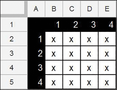
Figure 12.2 Possibility grid
Here you can see that if you list all objects in a row and also in a column, you can check off how many combinations there will be; this is the same as multiplying the number times itself, or finding the square. In this case, 4 squared is 16, so there are 16 combinations. This seems like a lot of combinations needed to do a comparison with just 4 objects, and indeed it is. There are several redundancies in the simplistic view of squaring the number that you can immediately eliminate. The first of which is a game object compared to itself. You don’t need to compare identical cars to know that they are the same, for example. If you look at every point where you would compare an object to itself, you find the clear pattern illustrated in Figure 12.3.
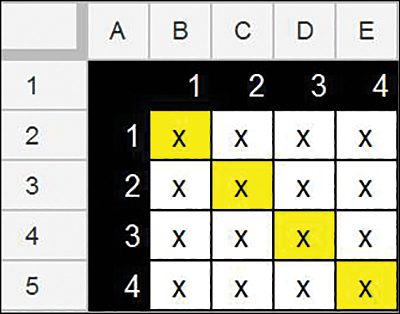
Figure 12.3 Unneeded combinations
Object 1 is compared to itself in cell B2, Object 2 is compared to itself in cell C3, and so on in a diagonal pattern through the chart. In a fighting game, you know that Combatant 1 will be equal to Combatant 1, so you can eliminate the need to test that combination. Therefore, you can eliminate every point on the graph where an object would be compared directly to itself. In the case shown in Figure 12.3, this is 4 combinations. In fact, for any comparison, the number of eliminations will equal the number of objects you are comparing. So, if you were to compare 6 objects, you could eliminate 6 combinations, and if you were to compare 1,000 objects, we could eliminate 1,000 combinations. With this in mind, you need to update your formula to get rid of those unneeded combinations. This is the update formula:
(Number of game objects)2 – (Number of game objects) = Unique comparisons
or:
G2 – G = Unique comparisons
or, in this example:
42 – 4 = 16 – 4 = 12 unique comparisons
While this formula removes the redundancy of comparing objects to themselves, there is one more step you can take to make your comparisons fully efficient. In a fighting game, if you compare Combatant 1 with Combatant 2, do you then need to compare Combatant 2 with Combatant 1? No. You already did that comparison, but in the opposite order, and because order doesn’t matter in the comparison, you can eliminate any combinations that you have already done in the opposite order. Figure 12.4 shows this graphically in a spreadsheet.
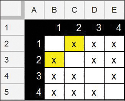
Figure 12.4 Redundant combinations
Both highlighted cells in Figure 12.4 are making the same comparison because they are both comparing object 1 with object 2, and you need only one of these comparisons. You need to know mathematically how many of these redundant comparisons are left in the chart. Because you are comparing every object with every other object, and all the objects are listed in both dimensions of the chart, you will get twice as many matchups of each object as needed. For every time Object 1 is compared to Object 2, Object 2 will be compared to Object 1. The same goes for each other pairing. This means you can eliminate half of the pairings because they are comparing the same two objects but in the opposite order. Figure 12.5 shows the redundant comparisons that you can eliminate.

Figure 12.5 Removing redundancies
Because all the highlighted cells in Figure 12.5 are redundant, you can remove them from your count of combinations that you need to test and balance. Mathematically, this means you can divide your total combinations by 2. This leads to the final formula:
(G2 – G)/2 = Total combinations to test
or, in this case:
(42 – 4)/2 = 6
To validate that the formula is working, you can count the number of Xs in your chart after eliminating all redundant combinations (see Figure 12.6).
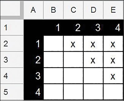
Figure 12.6 Valid remaining combinations
As you can see, 6 is indeed the number of valid combinations remaining. Now that you have the needed formula, you can input any number into it and find out exactly the number of combinations you need to compare your entire set of objects. As one more example, Figure 12.7 shows 20 objects and the combinations you need to test.
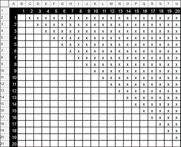
Figure 12.7 Large set of combinations
You can see that no matter how large or small the number of objects, the pattern repeats. If you plug in the new number to the formula, you get the following:
(202 – 20)/2 = 190 combinations
If you wanted, you could count the number of Xs in the chart and arrive at the same answer to verify, but doing so would take more time than using the combination formula. There is another way to do this formula that takes a little longer but that shows a very interesting pattern. To illustrate, let’s solve for the numbers 1 through 20 (see Table 12.14).
Notice that if you add the number of objects with the number of combinations, you get the number of combinations for the next greater count of objects. This means that if you know the formula for any number, you can quickly figure out the result for the next larger number by adding the number of objects to the number of combinations. If you wanted to extend this chart up to 21, therefore, you would add 20 to 190, for a result of 210 combinations.
When you know the number of combinations you are dealing with, you can use this information to more accurately calculate how much effort will be needed to check and balance these combinations. For example, if you know that it takes an hour to properly test and tune a single combination, you can figure out how many hours you need to account for in total.
Table 12.14 Possible combinations
Objects |
Combinations |
|---|---|
2 |
1 |
3 |
3 |
4 |
6 |
5 |
10 |
6 |
15 |
7 |
21 |
8 |
28 |
9 |
36 |
10 |
45 |
11 |
55 |
12 |
66 |
13 |
78 |
14 |
91 |
15 |
105 |
16 |
120 |
17 |
136 |
18 |
153 |
19 |
171 |
20 |
190 |
In addition to using the combinations formula for testing and balancing, you can use it in the following ways:
To make a round-robin tournament where every player plays every other player
In a fighting game, to create a special victory animation for each combination of combatants
In a racing game where a voiceover announcer says a unique line for each pairing of cars before the cars start the race
In a superhero game where two of heroes combine their powers to form a special power that is unique to that combination of characters
In a fantasy RPG, where each combination of character classes has a unique bonus when played as a team
In a combat game, to create a special animation for each combination of attack and defense
In addition to using the combinations formula to manually figure out how many combinations you need to test, you can use a spreadsheet shortcut function that does this math for you. This function, COMBIN, takes two arguments: the number of objects in the dataset and the number of objects in a combination. For all of the examples in this section, that second argument has been 2 because we have been combining only two objects at a time. However you can combine more than two objects with one another to get a significantly larger number of total combinations. Using a spreadsheet formula makes it possible to easily calculate these larger numbers of combinations.
Further Steps
After completing this chapter, you should take some time to practice in the real world with the concepts covered here. Try these exercises to further explore concepts covered in this chapter:
For some real-world examples of game objects, list their attributes and try to assign weights to those attributes. Try to do this for a variety of different objects and use the objects that you have created from previous chapters.
Create a naming convention for game objects—either objects you have made or preexisting games objects. Take the time to figure out how many attributes need to be contained in a name and in what order they should appear.
Use the handshake formula to determine the number of combinations in several actual scenarios (for example, your favorite upcoming sport or a game tournament you follow).