7.1 Existence and uniqueness theorem and main proprieties of the solution

Let be a complete probability space and a standard Wiener process defined on it. Let be a non‐anticipative filtration. Let be a ‐measurable r.v. (therefore independent of the Wiener process); in particular, it can be a deterministic constant. Having defined in Chapter  the Itô stochastic integrals, the stochastic integral equation

(7.1)

does have a meaning for if, as in Definition 6.4 of an Itô process,

Of course we need to impose appropriate conditions on and to insure that and , so that the integral form 7.1 has meaning and so the corresponding (Itô) stochastic differential equation (SDE)

(7.2)

also has a meaning for .

Besides having a meaning, we also want the SDE 7.2 to have a unique solution and this may require appropriate conditions for and . Like ordinary differential equations (ODEs), a restriction on the growth of these functions will avoid explosions of the solution (i.e. avoid the solution to diverge to in finite time) and a Lipschitz condition will insure uniqueness of the solution.

We will denote by the set of real‐valued functions with domain that are Borel‐measurable jointly in and ¹ and, for some and all and , verify the two properties:

• (Lipschitz condition)
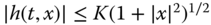• (restriction on growth).

We will follow the usual convention of not making explicit the dependence of random variables and stochastic processes on chance , but one should keep always in mind that such dependence exists and so the Wiener process and the solutions of SDE do depend on .

We now state an existence and uniqueness theorem for SDEs which is, with small nuances, the one commonly shown in the literature. Note that the conditions stated in the theorem are sufficient (not necessary), so there may be some improvements (i.e. the class of functions for which existence and uniqueness is insured may be enlarged), particularly in special cases. We will talk about that later.

Of course the starting time was labelled 0 and we will work on a time interval just for convenience, but nothing prevents one from working on intervals like .

Although further complications arise in the stochastic case, the theorem and the proof are inspired on an analogous existence and uniqueness theorem for ODEs. Both use the technique of proving uniqueness by assuming two solutions and showing they must be identical. Both use the constructive Picard's iterative method of approximating the solution by feeding one approximation into the integral equation to get the next approximation:

This method, which is very convenient for the proof, can be used in practice to approximate the solution, although it is quite slow compared to other available methods.

Monte Carlo simulation of SDEs

Although a more complete treatment will be presented in Section 12.2, we mention here some ideas on how to simulate trajectories of the solution of an SDE.

If an explicit expression for the solution of the SDE can be obtained, it can be used to simulate trajectories of . If the explicit expression only involves the Wiener process directly at the present time, we can simulate the Wiener process by the method of Section 4.1 and plug the values into the expression, as we will do to simulate the solution of the Black–Scholes model in Section 8.1. Monte Carlo simulation for more complicated explicit expressions will be addressed in Section  12.2 .

Unfortunately, in many cases we are unable to obtain an explicit expression, in which case the trajectories can be simulated using an approximation of obtained by discretizing time. One uses a partition of with a sufficiently large to reduce the numerical error. Typically, but not necessarily, the partition points are equidistant, with . A trajectory is simulated iteratively at the partition points. One starts (step 0) simulating by using the distribution of ; if is a deterministic value, then and no simulation is required. At each iteration (step with ), one uses the previously simulated value to simulate the next value . The simplest method to do that is the Euler method, the same as is used for ODEs. In the context of SDEs, it is also known as the Euler–Maruyama method. In this method, and are approximated in the interval by constants, namely by the values they take at the beginning point of the interval (to ensure the non‐antecipative property of the Itô calculus). This leads to the first‐order approximation scheme

Since the approximate value of is known from the previous iteration, the only thing random in the above scheme is the increment . The increments () are easily simulated (we have done this in Section  4.1 when simulating trajectories of the Wiener process), since they are independent random variables having a normal distribution with mean zero and variance . At the end of the iterations, we have the approximate values at the time partition points of a simulated trajectory. Of course, this iterative procedure can be repeated to produce other trajectories.

There are faster methods (i.e. requiring not so large values of ), like the Milstein method. On the numerical resolution/simulation of SDE, we refer the reader to Kloeden and Platen (1992), Kloeden et al. (1994), Bouleau and Lépingle (1994), and Iacus (2008).

SDE existence and uniqueness theorem

7.2 Proof of the existence and uniqueness theorem

We now present a proof of the existence and uniqueness Theorem 7.1, which can be skipped by non‐interested readers. Certain parts of the proof are presented in a sketchy way; for more details, the reader can consult, for instance, Arnold (1974), Øksendal (2003), Gard (1988), Schuss (1980) or Wong and Hajek (1985).

(a) Proof of uniqueness

Let and be two a.s. continuous solutions. They satisfy 7.4 and so are non‐anticipative (only depend on past values of themselves and of the Wiener process). Since and are Borel measurable functions, , , and are non‐anticipative. We could work with , but we have not yet proved that such second‐order moment indeed exists. So we replace it by the truncated moment , with if and for all and otherwise. Note that is non‐anticipative, that , and that for . Since and satisfy 7.4 , using the inequality , one gets

Using the Schwarz inequality (which, in particular, implies ), the fact that , and the norm preservation property for Itô integrals of functions, one gets

Putting and using the Lipschitz condition, one has

(7.6)

Using the Bellman–Gronwall lemma,⁴ also known as Gronwall's inequality, one gets , which implies a.s. But

and since are are a.s. bounded in (due to their a.s. continuity), both probabilities on the right‐hand side become arbitrarily small for every sufficiently large . So, a.s. for , and so also for all (since the set of rational numbers is countable). Due to the continuity, we have a.s. for all and therefore a.s.

(b) Proof of existence

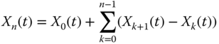
The proof of existence is based on the same Picard's method that is used on a similar proof for ODEs. It is an iterative method of successive approximations, starting with

(7.7)

and using the iteration

(7.8)

We just need to prove that () are a.s. continuous functions and that this sequence uniformly converges a.s. The limit will then be a.s. a continuous function, which, as we will show, is the solution of the SDE.

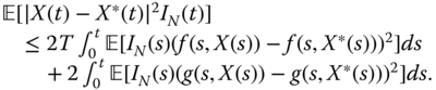
Since , we have and will see by induction that and for all . In fact, assuming this is true for , we show it is true for because (due to the restriction on growth, the norm preservation of the Itô integral, the inequality , and the Schwarz's inequality), with ,

(7.9)

Using a reasoning similar to the one used in the proof of 7.6, but now with no need to used truncated moments (since the non‐truncated moments exist), one obtains

(7.10)

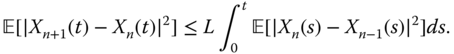
Iterating 7.10, one obtains by induction

Using the restriction on growth, one obtains

and so

Since

using (6.27) and the Lipschitz condition, one gets

By Thebyshev inequality,

By the Borel–Cantelli lemma,

and so, for every sufficiently large , a.s. Since the series is convergent, the series converges uniformly a.s. on (notice that the terms are bounded by ). Therefore

converges uniformly a.s. on .

This shows the a.s. uniform convergence of on as . Denote the limit by . Since are obviously non‐anticipative, the same happens to . The a.s. continuity of the and the uniform convergence imply the a.s. continuity of . Obviously, from the restriction on growth and a.s. continuity of , we have a.s. and a.s. Consequently, is an Itô process and the integrals in 7.4 make sense.

The only thing missing is to show that is indeed a solution, i.e. that satisfies 7.4 for . Apply limits in probability to both sides of 7.8. The left side converges in probability to (the convergence is even a stronger a.s. uniform convergence). On the right‐hand side, we have:

• The integrals converge a.s., and so converge in probability to . In fact, a.s. (due to the Lipschitz condition).
• The integrals converge to in probability. In fact, the Lipschitz condition implies a.s. and we can use the result of Exercise 6.9 in Section 6.4.
• So, the right‐hand side converges in probability to

Since the limits in probability are a.s. unique, we have

i.e. satisfies 7.4 .

Proof that and

From 7.9, putting gives . Iterating, we have

and therefore . Letting , by the dominated convergence theorem, we get

(7.11)

Consequently, and .

Proof that and are in

From the previous result, and , and so and are in .

As a consequence, the stochastic integral is a martingale.

Proof of 7.5

By the Itô formula (6.37),

(7.12)

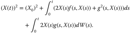
Applying mathematical expectations, one gets

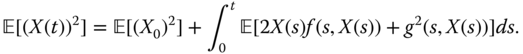
We have assumed that the stochastic integral has a null expected value, although we have not shown that the integrand function was in . Since this may fail, we should, in good rigour, have truncated by (to ensure the nullity of expectation of the stochastic integral) and then go to the limit as .

Using the restriction on growth and the inequality , one gets

Put and , note that and apply Gronwall's inequality to obtain , and so the first inequality of 7.5 .

From 7.4 , squaring and applying mathematical expectations, one gets

Applying the first expression of 7.5 and bounding the that shows up in the integral by , one gets the second expression in 7.5 .

Proof that the solution is m.s. continuous

For , is also solution of . Since now the initial condition is the value at time and the length of the time interval is , the second inequality in 7.5 now reads

(7.13)

and we can now use the first inequality of 7.5 to bound by . We conclude that as , which proves the m.s. continuity.

Proof of the semigroup property: For ,

This is an easy consequence of the trivial property of integrals (if one splits the integration interval into two subintervals, the integral over the interval is the sum of the integrals over the subintervals), which gives .

Proof that the solution is a Markov process

Let . The intuitive justification that is a Markov process comes from the semigroup property . This means that can be obtained in the interval as solution of . So, given , is defined in terms of and (), and so is measurable with respect to . Since is ‐measurable, and so is independent of , we conclude that, given , only depends on . Since is independent of , also (future value) given (present value) is independent of (past values). Thus, it is a Markov process.

A formal proof can been seen, for instance, in Gihman and Skorohod (1972), Arnold (1974), and Gard (1988).

Proof that, if and are also continuous in , then is a diffusion process

Let and . Conditioning on (deterministic initial condition), from 7.13 we obtain

(7.14)

First of all, let us note that expressions similar to 7.5 can be obtained for higher even ‐order moments if . Therefore, since now the initial condition is deterministic and so has moments of any order , we can use such expressions to obtain expressions of higher order similar to 7.14. We get

(7.15)

with and appropriate positive constants. Given , since , we get

Due to 7.15, these moments exist for all (even for odd , the moment exists since the moment of order exists). Since is a Markov process with a.s. continuous trajectories, we just need to show that (5.1), (5.2), and (5.3) hold.

Due to the Lipschitz condition, notice that and are also continuous functions of .

From 7.15 with we get , with constant, so that as Therefore

So, (5.1) holds.

Starting from 7.4 , since the Itô integral has zero expectation, we get

(7.16)

We also have, using the Lipschitz condition, Schwarz's inequality, and 7.14 ,

(7.17)

where is a positive constant that does not depend on . The continuity of in holds on the close interval and is uniform. Therefore, given an arbitrary , there is a independent of such that

(7.18)

From 7.16, 7.17, and 7.18, we obtain (5.2) with .

To obtain (5.3) with , one starts from 7.12 instead of 7.4 , using also as initial condition and applying similar techniques.

This concludes the proof of Theorem 7.1.

7.3 Observations and extensions to the existence and uniqueness theorem

The condition (i.e. has finite variance) is really not required and we could prove Theorem 7.1, with the exception of parts (c) and (d), without making that assumption. Of course, for parts (c) and (d) we would need the assumption, since otherwise the required second‐order moments of might not exist.

In fact, except for parts (c) and (d), we could easily adapt the proof presented in Section 7.2 in order to wave that assumption. We would just replace by its truncation to an interval . Since the truncated r.v. is in , the proof would stand for the truncated , and then we would go to the limit as .

The restriction to growth and the Lipschitz condition for and do not always need to hold for all points , or and . In the case where the solution of the SDE has values that always belong to a set , then it is sufficient that the restriction on growth and the Lipschitz conditions are valid on . In fact, in that case nothing changes if we replace and by other functions that coincide with them on and have zero values out of , and these other functions satisfy the restriction on growth and the Lipschitz condition.

For existence and uniqueness, we could use a weaker local Lipschitz condition for and instead of the global Lipschitz condition we have assumed in Theorem 7.1.

A function with domain satisfies a local Lipschitz condition if, for any , there is a such that, for all and , , we have

(7.19)

The proof of existence uses a truncation of to the interval and ends by taking limits as .

Consider and fixed. We can say that the SDE , , or the corresponding stochastic integral equation , is a map (or transformation) that, given a r.v. and a Wiener process (on a certain given probability space endowed with a non‐anticipative filtration ), transforms them into the a.s. unique solution of the SDE, which is adapted to the filtration. If we choose a different Wiener process, the solution changes. This type of solution, which is the one we have studied so far, is the one that is understood by default (i.e. if nothing in contrary is said). It is called a strong solution. Of course, once the Wiener process is chosen, the solution is unique a.s. and to each there corresponds the value of and the whole trajectory of the Wiener process, which the SDE (or the corresponding stochastic integral equation) transforms into the trajectory of the SDE solution. In summary, and the Wiener process are both given and we seek the associated unique solution of the SDE.

There are also weak solutions. Again, consider and fixed. Now, however, only is given, not the Wiener process. What we seek now is to find a probability space and a pair of processes and on that space such that ; of course, these are not unique. The difference is that, in the strong solution, the Wiener process is given a priori and chosen freely, the solution being dependent on the chosen Wiener process, while in the weak solution, the Wiener process is obtained a posteriori and is part of the solution.⁵ Of course, a strong solution is also a weak solution, but the reverse may fail. One can see a counter‐example in Øksendal (2003), in which the SDE has no strong solutions but does have weak solutions.

The uniqueness considered in Theorem 7.1 is the so‐called strong uniqueness, i.e. given two solutions, their sample paths coincide for all with probability one. We also have weak uniqueness, which means that, given two solutions (no matter if they are weak or strong solutions), they have the same finite‐dimensional distributions. Of course, strong uniqueness implies weak uniqueness, but the reverse may fail. Under the conditions assumed in the existence and uniqueness Theorem 7.1, two weak or strong solutions are weakly unique. In fact, given two solutions, either strong or weak, they are also weak solutions. Let them be and (remember that a weak solution is a pair of the ‘solution itself’ and a Wiener process). Then, since by the theorem there are strong solutions, let and be the strong solutions corresponding to the Wiener process choices and . By Picard's method of successive approximations given by 7.7– 7.8 , the approximating sequences have the same finite‐dimensional distributions, so the same happens to their a.s. limits and .

It is important to stress that, under the conditions assumed in the existence and uniqueness Theorem 7.1, from the probabilistic point of view, i.e. from the point of view of finite‐dimensional distributions, there is no difference between weak and strong solutions nor between the different possible weak solutions. This may be convenient since, to determine the probabilistic properties of the strong solution, we may work with weak solutions and get the same results.

Sometimes the Lipschitz condition or the restriction on growth are not valid and so the existence of strong solution is not guaranteed. In that case, one can see if there are weak solutions. Conditions for the existence of weak solutions can be seen in Stroock and Varadhan (2006) and Karatzas and Shreve (1991). Another interesting result is (see Karatzas and Shreve (1991)) that, if there is a weak solution and strong uniqueness holds, then there is a strong solution.

We have seen that, when and , besides satisfying the other assumptions of the existence and uniqueness Theorem 7.1, were also continuous functions of time, the solution of the SDE was a diffusion process with drift coefficient and diffusion coefficient .

The reciprocal problem is also interesting. Given a diffusion process () in a complete probability space with drift coefficient and diffusion coefficient , is there an SDE which has such a process as a weak solution? Under appropriate regularity conditions, the answer is positive. Some results on this issue can be seen in Stroock and Varadhan (2006), Karatzas and Shreve (1991), and Gihman and Skorohod (1972). So, in a way, there is a correspondence between solutions of SDE and diffusion processes.

In the particular case that and do not depend on time (and satisfy the assumptions of the existence and uniqueness Theorem 7.1), they are automatically continuous functions of time and therefore the solution of the SDE will be a homogeneous diffusion process with drift coefficient and diffusion coefficient . In this case, the SDE is an autonomous stochastic differential equation and its solution is also called an Itô diffusion. In this case, one does not need to verify the restriction on growth assumption since this is a direct consequence of the Lipschitz condition (this latter condition, of course, needs to be checked). In the autonomous case, one can work in the interval since and do not depend on time.

In the autonomous case, under the assumptions of the existence and uniqueness Theorem 7.1, one can even conclude that the solution of the SDE is a strong Markov process (see, for instance, Gihman and Skorohod (1972) or Øksendal (2003)).

In the autonomous case, if we are working in one dimension (so this is not generalizable to multidimensional SDEs), we can get results even when the Lipschitz condition fails but and are continuously differentiable (i.e. are of class ). Note that, if they are of class , they may or may not verify a Lipschitz condition; if they have bounded derivatives, they satisfy a Lipschitz condition, but this is not the case if the derivatives are unbounded.

The result by McKean (1969) for autonomous one‐dimensional SDEs is that, if and are of class , then there is a unique (strong) solution up to a possible explosion time . By explosion, we mean the solution becoming . If and also satisfy a Lipschitz condition, that is sufficient to prevent explosions (i.e. one has a.s.) and the solution exists for all times and is unique. If and are of class but fail to satisfy a Lipschitz condition, one cannot exclude the possibility of an explosion, but there are cases in which one can show that an explosion is not possible (or, more precisely, has a zero probability of occurring) and therefore the solution exists for all times and is unique. We will see later some examples of such cases and of the simple methods used to show that in such cases there is no explosion. There is also a test to determine whether an explosion will or will not occur, the Feller test (see McKean (1969)).

Let us now consider multidimensional stochastic differential equations. The setting is similar to that of the multidimensional Itô processes of Section 6.7. The difference is that now one uses and . The Lipschitz condition and the restriction on growth of and in the existence and uniqueness Theorem 7.1 are identical with representing the euclidean distance. The results of Theorem 7.1 remain valid. When the solution is a diffusion process, the drift coefficient is the vector and the diffusion coefficient is the matrix .

Notice, however, that, given a multidimensional diffusion process with drift coefficient and diffusion coefficient , there are several matrices for which , but all of them result in the same probabilistic properties for the solution of the SDE. So, from the point of view of probabilistic properties or of weak solutions, it is irrelevant which one chooses.

The treatment in this chapter allows the inclusion of SDE of the type

by adding the equation and working in two dimensions with the vector and the SDE

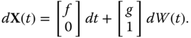
The initial condition takes the form . Note that and .

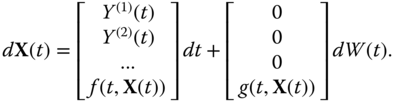
We can also have higher order stochastic differential equations of the form (here the superscript represents the derivative of order )

with initial conditions (). For that, we use the same technique that is used for higher order ODEs, working with the vector

and the SDE

We can also have functions and that depend on chance in a more general direct way (thus far they did not depend directly on chance, but they did so indirectly through ). This poses no problem as long as and are kept non‐anticipative.