10
Heat Transfer
10.1 Introduction
In this chapter we develop the variational formulation to model the steady‐state heat transfer in rigid continuum media, that is, in bodies where the spatial position of particles remains invariant.
According to the roadmap established in Chapter 3, the first step in the construction of a variational model consists of defining the kinematics for the model, that is, the motion actions that particles can execute. In the heat transfer problem, the temperature is the primary scalar field that characterizes the average kinetic energy of molecules, and so it characterizes the kinematics in this problem. The temperature in a body is constrained to satisfy certain conditions, and therefore it is possible to define the concept of admissible variations of the temperature fields. With this, it is possible to introduce the generalized strain action operator, which in this context is denoted by ![]() (in Chapter 3 it was denoted by
(in Chapter 3 it was denoted by ![]() ), which leads us to the conception of the virtual internal power. From there, the characterization of generalized internal and external forces will follow, and then the application of the Principle of Virtual Power will be exploited to define the concept of equilibrium for the system.
), which leads us to the conception of the virtual internal power. From there, the characterization of generalized internal and external forces will follow, and then the application of the Principle of Virtual Power will be exploited to define the concept of equilibrium for the system.
Let us consider a body occupying a bounded and regular region ![]() 1, with boundary
1, with boundary ![]() , in the three‐dimensional Euclidean space
, in the three‐dimensional Euclidean space ![]() . As a consequence, spatial coordinates
. As a consequence, spatial coordinates ![]() coincide with the material (reference) coordinates
coincide with the material (reference) coordinates ![]() admitted for the particles. That is, the spatial configuration and the material configuration of the body agree. For the heat transfer problem in bodies whose deformations are substantial, the developments of this chapter remain valid, but the reader has to keep in mind that the configuration of the body referred to in what follows is the spatial (actual, deformed) configuration the body occupies in space once the mechanical equilibrium has been achieved.
admitted for the particles. That is, the spatial configuration and the material configuration of the body agree. For the heat transfer problem in bodies whose deformations are substantial, the developments of this chapter remain valid, but the reader has to keep in mind that the configuration of the body referred to in what follows is the spatial (actual, deformed) configuration the body occupies in space once the mechanical equilibrium has been achieved.
10.2 Kinematics
Making the analogy with the velocity field in the mechanics of continuum media, the scalar field called temperature, and denoted by ![]() , becomes the primal (also primary) variable in the heat transfer problem.2
, becomes the primal (also primary) variable in the heat transfer problem.2

Figure 10.1 Spatial configuration of the body for the heat transfer problem.
We call ![]() the set of all possible temperature scalar fields that are sufficiently regular and can be defined over the body
the set of all possible temperature scalar fields that are sufficiently regular and can be defined over the body ![]() . Here, the set
. Here, the set ![]() , endowed with the usual operations of addition and multiplication by a real number, becomes a vector space. By regular it is understood that
, endowed with the usual operations of addition and multiplication by a real number, becomes a vector space. By regular it is understood that ![]() is smooth enough such that all operations to be executed over this field are well‐defined.
is smooth enough such that all operations to be executed over this field are well‐defined.
Consider that there exists a portion of the boundary, called ![]() , where the temperature is prescribed. Then, we define the set
, where the temperature is prescribed. Then, we define the set
where ![]() is the value of the prescribed temperature on
is the value of the prescribed temperature on ![]() , as illustrated in Figure 10.1.
, as illustrated in Figure 10.1.
The set ![]() contains all admissible temperature fields for the problem under study. Moreover, we define the vector subspace associated with
contains all admissible temperature fields for the problem under study. Moreover, we define the vector subspace associated with ![]() with fields satisfying homogeneous boundary conditions on
with fields satisfying homogeneous boundary conditions on ![]() , that is
, that is
It is easy to verify that ![]() is the translation of the subspace
is the translation of the subspace ![]() . The elements
. The elements ![]() are called virtual thermal variations, or admissible temperature variations. With the previous elements we can write
are called virtual thermal variations, or admissible temperature variations. With the previous elements we can write
where ![]() is arbitrary. Now, consider that the regularity of the temperature fields is such that we can express the temperature at a point
is arbitrary. Now, consider that the regularity of the temperature fields is such that we can express the temperature at a point ![]() close to
close to ![]() using a Taylor expansion as follows
using a Taylor expansion as follows
Calling ![]() to the vector field
to the vector field ![]() and for all points
and for all points ![]() in a sufficiently small neighborhood of
in a sufficiently small neighborhood of ![]() we can admit that the following holds
we can admit that the following holds
In addition, the field ![]() is called constant, or rigid, if it verifies
is called constant, or rigid, if it verifies
or equivalently
Thus, another fundamental ingredient in the present model is the vector field ![]() which represents the temperature spatial gradient (or thermal gradient). In particular, the set of all sufficiently regular fields
which represents the temperature spatial gradient (or thermal gradient). In particular, the set of all sufficiently regular fields ![]() is denoted by
is denoted by ![]() .
.
We will say that ![]() is a thermal gradient, or compatible gradient, if it is possible to determine
is a thermal gradient, or compatible gradient, if it is possible to determine ![]() such that
such that
Thus, we can define the operator ![]() which for each
which for each ![]() assigns a thermal gradient
assigns a thermal gradient ![]() .
.
The kernel of operator ![]() , denoted by
, denoted by ![]() , is then characterized by
, is then characterized by
and consists of all rigid thermal actions. All the elements and kinematical concepts introduced so far have a full parallel with the fundamental ingredients introduced in Chapter 3.
10.3 Principle of Thermal Virtual Power
As in the mechanics of continuum media, let us admit that external thermal loads that exert some action over the body ![]() are characterized by linear (and continuous) functionals
are characterized by linear (and continuous) functionals ![]() . Hence, the external thermal loads are elements of the space dual to
. Hence, the external thermal loads are elements of the space dual to ![]() , here represented by
, here represented by ![]() . We will call the value this functional takes in
. We will call the value this functional takes in ![]() the external thermal power, which is then given by
the external thermal power, which is then given by
where ![]() is the duality product
is the duality product ![]() .
.
In this section we will see that these external thermal loads can be explicitly characterized by making use of the Principle of Thermal Virtual Power, which will be enunciated next.
First, let us define the internal thermal stresses through proper linear (and continuous) functionals defined over the space of temperatures ![]() and of thermal gradients
and of thermal gradients ![]() . The value taken by such functionals at point
. The value taken by such functionals at point ![]() is termed the internal thermal power, or simply
is termed the internal thermal power, or simply ![]() . Once again, as in the mechanics domain, we will introduce a series of hypotheses that will allow us to find a representation for such a functional.
. Once again, as in the mechanics domain, we will introduce a series of hypotheses that will allow us to find a representation for such a functional.
First, let us assume that the functional has the following general representation
The second hypothesis corresponds to admitting that ![]() is null for all rigid thermal actions (uniform
is null for all rigid thermal actions (uniform ![]() ), that is
), that is

which yields

Since the expression above must hold for every part ![]() of the body
of the body ![]() , it implies
, it implies
Thus, we have

With this procedure, we have arrived at a duality between the thermal gradient and the heat flux.3
We then conclude that internal thermal stresses are linear (and continuous) functionals defined over ![]() , that means they are elements in the space dual to
, that means they are elements in the space dual to ![]() , here designated by
, here designated by ![]() . By virtue of the Riesz representation theorem we can put these functionals in correspondence with a vector field, say
. By virtue of the Riesz representation theorem we can put these functionals in correspondence with a vector field, say ![]() , which is named as the heat flux vector field. Therefore, the value of this functional at
, which is named as the heat flux vector field. Therefore, the value of this functional at ![]() is given by
is given by

We have then defined the spaces ![]() ,
, ![]() ,
, ![]() and
and ![]() and the dual products (linear forms)
and the dual products (linear forms) ![]() and
and ![]() which provide a correspondence between these spaces. Now, we define the adjoint operator
which provide a correspondence between these spaces. Now, we define the adjoint operator ![]() , called the thermal equilibrium operator, as
, called the thermal equilibrium operator, as
At this stage we have all the elements required to formalize the variational principle which rules the problem, and which we call the Principle of Thermal Virtual Power (PTVP). Then, we say that a body ![]() , under the action of the external thermal loads
, under the action of the external thermal loads ![]() , is at static4 thermal equilibrium if
, is at static4 thermal equilibrium if
which implies that the external thermal virtual power is nullified for all rigid thermal actions and, in addition, satisfies
that is, the sum of the internal thermal virtual power and of the external thermal virtual power equals zero for all admissible virtual thermal actions.
The first part of the PTVP enables us to establish which are the external thermal loads compatible with the thermal equilibrium. Note that this first part makes sense provided the existence of ![]() for a given
for a given ![]() at equilibrium is demonstrated. This is, in fact, the reason to show the following result.
at equilibrium is demonstrated. This is, in fact, the reason to show the following result.
According to the previous results we conclude that
which means
Hence, the theorem 10.1 and the concept of equilibrium for rigid thermal actions allow us to obtain the second part of the PTVP.
In this manner, we arrived at the point in which we have been given all the necessary elements to formulate the variational equations and retrieve from them the associated Euler–Lagrange equations which govern the steady‐state heat transfer problem in strong form. Hereafter, we will provide a more concrete notation to these ingredients, specifying the context of three‐dimensional heat transfer with ![]() . Therefore, from the PTVP we have
. Therefore, from the PTVP we have

If ![]() and
and ![]() are sufficiently regular fields, we can integrate by parts as follows
are sufficiently regular fields, we can integrate by parts as follows

where we have used the fact that ![]() over
over ![]() , where
, where ![]() with
with ![]() (see Figure 10.1).
(see Figure 10.1).
Placing (10.31) into expression (10.30) provides the characterization for the element ![]()

This result tells us that the external thermal loads compatible with the kinematical model consist of a thermal load per unit volume, denoted by ![]() , and a thermal load per unit area, denoted by
, and a thermal load per unit area, denoted by ![]() .
.
In diverse applications of practical interest, where the material surrounding the solid body is a flowing fluid, the load ![]() depends upon the temperature of the solid boundary,
depends upon the temperature of the solid boundary, ![]() , of the fluid temperature at remote locations, say
, of the fluid temperature at remote locations, say ![]() , and of the properties of the fluid and of the type of surface, lumped into a parameter
, and of the properties of the fluid and of the type of surface, lumped into a parameter ![]() , through a relation
, through a relation ![]() . We call this physical phenomenon the convective heat exchange, and the surface where this exchange takes place is denoted
. We call this physical phenomenon the convective heat exchange, and the surface where this exchange takes place is denoted ![]() . If we consider
. If we consider ![]() we obtain the following representation for
we obtain the following representation for ![]()

Then, the PTVP consists of the variational equation

To extend the PTVP to the case of unsteady heat transfer it is enough to replace ![]() by
by ![]() where
where ![]() is the density for the material in
is the density for the material in ![]() and
and ![]() is the specific heat, being
is the specific heat, being ![]() in the case of solids.
in the case of solids.
Thus, in order to find the local form of the variational problem (10.34) we have to find the associated Euler–Lagrange equations, whose abstract form is ![]() as we have seen in (10.20). We proceed with the integration by parts for the left‐hand side of equation (10.34), yielding
as we have seen in (10.20). We proceed with the integration by parts for the left‐hand side of equation (10.34), yielding

Using now standard variational arguments (fundamental theorem of the calculus of variations), we find
which are the Euler–Lagrange equations sought for the variational equation (10.34).
Notice that, even in situations in which the fields are not regular enough so that integration by parts can be safely performed as we did, the PTVP still holds. In this regard, consider, for example, that there exists an internal surface, say ![]() , which divides the body into two parts, each of which features smooth fields so that integration by parts can be pursued. In this case, from the integration by parts procedure emerges an additional term of the form
, which divides the body into two parts, each of which features smooth fields so that integration by parts can be pursued. In this case, from the integration by parts procedure emerges an additional term of the form ![]() . This indicates that the system of external thermal loads
. This indicates that the system of external thermal loads ![]() could account for a load per unit area defined over the internal surface
could account for a load per unit area defined over the internal surface ![]() , say
, say ![]() . Hence, the equilibrium in such case implies
. Hence, the equilibrium in such case implies
Let us now characterize the reactive flux ![]() by releasing the kinematical constraints from space
by releasing the kinematical constraints from space ![]() . To do this, note that (10.20) is equivalent to the following
. To do this, note that (10.20) is equivalent to the following
Using the PTVP yields

and, after integration by parts, it becomes

As a direct consequence, we have that
which, in local form, implies
The reactive flux ![]() is the normal component of the heat flux vector field over the part of the boundary in which the temperature has been constrained.
is the normal component of the heat flux vector field over the part of the boundary in which the temperature has been constrained.
Finally, the reader will find in Figure 10.2 the main concepts and results which characterize the variational formulation.

Figure 10.2 Ingredients in the variational theory for the heat transfer model.
10.4 Principle of Complementary Thermal Virtual Power
The previous section dealt with the primal variational form of the steady‐state heat transfer problem, characterized through the PTVP, which establishes a connection between the internal thermal stress ![]() and the external thermal load
and the external thermal load ![]() so that (steady‐state) equilibrium is achieved.
so that (steady‐state) equilibrium is achieved.
As in the mechanics of deformable bodies, for the heat transfer problem it is also possible to introduce a problem which can be regarded as dual to the primal problem, in the sense that it provides a characterization of the compatibility of the thermal gradient vector field ![]() , that is, to determine whether there exists
, that is, to determine whether there exists ![]() such that
such that ![]() . To formulate this problem we first define the following sets
. To formulate this problem we first define the following sets
which is the set of all internal thermal stresses that are equilibrated with the external thermal load ![]() , and
, and
which is the vector subspace of ![]() whose elements are internal thermal stresses (heat flux fields)
whose elements are internal thermal stresses (heat flux fields) ![]() at thermal equilibrium with the null thermal load.
at thermal equilibrium with the null thermal load.
As before, it is important to note that if ![]() and
and ![]() then
then
because
This result shows us that ![]() is a translation of
is a translation of ![]() , that is
, that is
With the previous definitions, we can now enunciate the Principle of Complementary Thermal Virtual Power (PCTVP). We say that the vector field ![]() is thermally compatible for an external thermal load
is thermally compatible for an external thermal load ![]() at equilibrium if and only if
at equilibrium if and only if
for some ![]() .
.
To see this result, consider first that ![]() is compatible, then
is compatible, then ![]() such that
such that ![]() . Since
. Since ![]() is a translation of
is a translation of ![]() , that is,
, that is, ![]() , with
, with ![]() arbitrary, we have
arbitrary, we have ![]() . Then
. Then
which results in the very definition of the space ![]() .
.
Suppose now that
where ![]() . Hence
. Hence
and we conclude that
Moreover, from (10.46) we also know that
and then
Replacing (10.56) into (10.54) yields
which means ![]() or, equivalently,
or, equivalently, ![]() such that
such that ![]() .
.
For the case under analysis, expression (10.50) corresponds to

so by making use of integration by parts we find

where we make use of the fact that ![]() in
in ![]() ,
, ![]() on
on ![]() and on
and on ![]() , and
, and ![]() on
on ![]() .
.
Therefore, we conclude that the PCTVP acquires the following variational form

10.5 Constitutive Equations
In our road towards the formulation of a field problem for the heat transfer problem there is still a missing aspect concerning the material behavior in the present context. This constitutive material response determines the way in which the heat flux ![]() is related to the thermal gradient
is related to the thermal gradient ![]() . That is, we have to look for an operator that maps the space
. That is, we have to look for an operator that maps the space ![]() into its dual
into its dual ![]() . A typical constitutive model is that given by a linear relation, which states that
. A typical constitutive model is that given by a linear relation, which states that
where ![]() is a second‐order tensor and the sign indicates that the heat flux opposes the thermal gradient. Next, we further assume that the tensor
is a second‐order tensor and the sign indicates that the heat flux opposes the thermal gradient. Next, we further assume that the tensor ![]() satisfies the following properties
satisfies the following properties
Let us now define the thermal gradient energy density function ![]() as
as

Notice that from the properties of ![]() it follows that
it follows that
where the equality is verified for ![]() .
.
Thus, the heat flux ![]() related to the thermal gradient
related to the thermal gradient ![]() through the constitutive equation is such that
through the constitutive equation is such that

In turn, a Taylor's expansion ![]() around the point
around the point ![]() provides
provides

which gives
while the equality is verified for ![]() . In this case we conclude that
. In this case we conclude that ![]() is a strictly concave function.
is a strictly concave function.
In the case of materials featuring nonlinear constitutive behavior we assume the following property for ![]() holds
holds
with the equality being valid for ![]() , and
, and ![]() ,
, ![]() . Let
. Let ![]() be a thermal gradient whose heat flux is
be a thermal gradient whose heat flux is ![]() . Then
. Then
and integrating the process that takes us from ![]() to
to ![]() we arrive at
we arrive at

and so we get
where we have recovered the concavity of function ![]() from the monotonicity property stated by (10.70).
from the monotonicity property stated by (10.70).
By virtue of the positive‐definiteness of tensor ![]() , we can calculate the inverse
, we can calculate the inverse ![]() , and we can find the inverse constitutive equation as follows
, and we can find the inverse constitutive equation as follows
therefore it is possible to introduce the complementary thermal gradient energy density function as
where the equality is verified for ![]() . Furthermore,
. Furthermore,

and also
which allows us to conclude that function ![]() is also concave in the space
is also concave in the space ![]() .
.
From the properties of ![]() and
and ![]() we verify that
we verify that
where the equality is satisfied if ![]() and
and ![]() are related by means of the constitutive equation.
are related by means of the constitutive equation.
10.6 Principle of Minimum Total Thermal Energy
The goal of this section is to transform the steady‐state heat transfer problem into a minimization problem with a corresponding cost functional. Therefore, we proceed analogously to the steps presented in Chapter 4.
Since function ![]() is concave, from (10.73) we can write
is concave, from (10.73) we can write
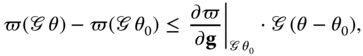
where the equality holds for all ![]() . Integrating (10.79) in the domain occupied by the body
. Integrating (10.79) in the domain occupied by the body ![]() , we obtain the following
, we obtain the following

Replacing this result into the PTVP expressed by equation (10.30) gives

Let us define the Total Thermal Energy as follows

then after arranging terms we get

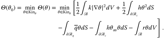
In this way, we have arrived at the Principle of Minimum Total Thermal Energy, which consists of finding ![]() that minimizes the Total Thermal Energy functional, that is
that minimizes the Total Thermal Energy functional, that is

10.7 Poisson and Laplace Equations
Consider the constitutive model most widely used in practice for this kind of problem. Such a model is known as the Fourier law and it establishes that the heat flux ![]() and the thermal gradient
and the thermal gradient ![]() are related as follows
are related as follows
where ![]() is characterized by a single (positive) scalar field
is characterized by a single (positive) scalar field ![]() , called the material thermal conductivity, and
, called the material thermal conductivity, and ![]() is the second‐order identity tensor.
is the second‐order identity tensor.
Then, we rewrite the PTVP given by (10.34) for the particular choice of a material ruled by constitutive equation (10.85)

The Euler–Lagrange equations are obtained by integrating by parts the left‐hand side in the above expression and using standard arguments from the calculus of variations
Let us further simplify the presentation for the case of thermally homogeneous materials, that is, for materials featuring a constant conductivity ![]() , and also for homogeneous essential boundary conditions over the whole boundary, that is,
, and also for homogeneous essential boundary conditions over the whole boundary, that is, ![]() over
over ![]() . Then, the problem is reduced to the widely known Poisson problem
. Then, the problem is reduced to the widely known Poisson problem
If now we consider a given ![]() over the boundary
over the boundary ![]() , and that
, and that ![]() , we arrive at the Dirichlet problem for the Laplace equation
, we arrive at the Dirichlet problem for the Laplace equation
which characterizes the so‐called harmonic functions.
Next, we present the variational problem (10.86) in the format of a minimization problem. Thus, and noting that for the Fourier law the thermal energy density function is given by
the total thermal energy functional (10.82) gives

Finally, after rearranging terms, the minimization problem standing from (10.84) amounts to finding ![]() such that
such that
Note that the term ![]() becomes quadratic when paired with
becomes quadratic when paired with ![]() , this gives rise to the term of the form
, this gives rise to the term of the form ![]() in the expression above. Here we have simplified the presentation by directly modifying the cost functional to account for this fact, and to ensure that the first Gâteaux derivative of functional
in the expression above. Here we have simplified the presentation by directly modifying the cost functional to account for this fact, and to ensure that the first Gâteaux derivative of functional ![]() in (10.95) actually corresponds to the variational equation (10.86). An alternative more systematic way to do this involves postulating that the internal energy is not only composed by
in (10.95) actually corresponds to the variational equation (10.86). An alternative more systematic way to do this involves postulating that the internal energy is not only composed by ![]() integrated over the body domain
integrated over the body domain ![]() , but also by a surface energy
, but also by a surface energy ![]() of the form
of the form ![]() , defined over the boundary
, defined over the boundary ![]() . In turn, the external system of body forces must include a heat flux of the form
. In turn, the external system of body forces must include a heat flux of the form ![]() .
.
Note
- 1 An additional hypothesis is that this region is spatially fixed.
- 2 In [242] the concept of thermal displacement
 is utilized in the development of the theory, whose relation with the temperature here is
  .
. - 3 Actually, the dual variable to the temperature, in the sense of mechanical power, is the so‐called entropy flux, denoted by
 . In the present development, since we are working with mechanical power per unit temperature, here simply called thermal power, the dual variable to the thermal gradient is, in fact, the heat flux, whose relation to the entropy flux is
  .
. - 4 We added this characterization because at the beginning of this chapter we tackled the steady‐state heat transfer problem. Extension to the unsteady case is straightforward and is also carried out in this section.