
Overview of Stepwise Regression
In JMP, stepwise regression is a personality of the Fit Model platform. The Stepwise feature computes estimates that are the same as those of other least squares platforms, but it facilitates searching and selecting among many models.
The approach has side effects of which you need to be aware. The significance levels on the statistics for selected models violate the standard statistical assumptions because the model has been selected rather than tested within a fixed model. On the positive side, the approach has been helpful for 30 years in reducing the number of terms. The book Subset Selection in Regression, by A. J. Miller (1990), brings statistical sense to model selection statistics.
This chapter uses the term significance probability in a mechanical way to represent that the calculation would be valid in a fixed model, recognizing that the true significance probability could be nowhere near the reported one.
Example Using Stepwise Regression
The Fitness.jmp (SAS Institute Inc. 1987) data table contains the results of an aerobic fitness study. Aerobic fitness can be evaluated using a special test that measures the oxygen uptake of a person running on a treadmill for a prescribed distance. However, it would be more economical to find a formula that uses simpler measurements that evaluate fitness and predict oxygen uptake. To identify such an equation, measurements of age, weight, run time, and pulse were taken for 31 participants who ran 1.5 miles.
Note: For purposes of illustration, certain values of MaxPulse and RunPulse have been changed from data reported by Rawlings (1988, p.105).
1. Select Help > Sample Data Library and open Fitness.jmp.
2. Select Analyze > Fit Model.
3. Select Oxy and click Y.
4. Select Weight, Runtime, RunPulse, RstPulse, MaxPulse, and click Add.
5. For Personality, select Stepwise.
Figure 5.1 Completed Fit Model Launch Window
6. Click Run.
Figure 5.2 Stepwise Report Window
To find a good oxygen uptake prediction equation, you need to compare many different regression models. Use the options in the Stepwise report window to search through models with combinations of effects and choose the model that you want.
The Stepwise Report
The Stepwise report window contains platform options, a regression control panel, current estimates, and step history.
Platform options
The red triangle menu next to Stepwise Fit contains options that affect all of the variables. See “Stepwise Platform Options”.
Stepwise Regression Control
Limits regressor effect probabilities, determines the method of selecting effects, starts or stops the selection process, and creates a model. See “Stepwise Regression Control Panel”.
Current Estimates
Enters, removes, and locks in model effects. See “Current Estimates Report”.
Step History
Records the effect of adding a term to the model. See “Step History Report”.
Stepwise Platform Options
The red triangle menu next to Stepwise Fit contains the following platform options.
K-Fold Crossvalidation
Performs K-Fold cross validation in the selection process. When selected, this option enables the Max K-Fold RSquare stopping rule (“Stepwise Regression Control Panel”).
Available only for continuous responses. For more information about validation, see “Using Validation”.
All Possible Models
Fits all possible models up to specified limits and shows the best models for each number of terms. Enter values for the maximum number of terms to fit in any one model. Also enter values for the maximum number of best model results to show for each number of terms in the model. Categorical variables are represented using indicator variables. See “Models with Nominal and Ordinal Effects”. You can restrict the models that appear to those that satisfy strong effect heredity. See “The All Possible Models Option”.
This option is available only for continuous responses.
Model Averaging
Enables you to average the fits for a number of models, instead of picking a single best model. See “The Model Averaging Option”.
Available only for continuous responses.
Plot Criterion History
Creates a plot of AICc and BIC versus the number of parameters. The Criterion History plot contains two shaded zones. Define the minimum AICc value as Vbest. The green zone is defined by the range [Vbest, Vbest+4]. The yellow zone is defined by the range (Vbest+4, Vbest+10].
Plot RSquare History
Creates a plot of training and validation R-square versus the number of parameters.
Available only for continuous responses.
Clear History
Clears and resets the step history.
Adds the Validation column to the Model Specification window when you select Make Model. Runs the model with the Validation column when you select Run Model.
This option is selected by default.
Note: This option appears only when you have entered a Validation column in the Stepwise launch window.
Model Dialog
Shows the completed launch window for the current model.
Stepwise Regression Control Panel
Use the Stepwise Regression Control panel to limit regressor effect probabilities, determine the method of selecting effects, begin or stop the selection process, and run a model. A note appears beneath the Go button to indicate if you have excluded or missing rows.
Figure 5.3 Stepwise Regression Control Panel
Stopping Rule
The Stopping Rule determines which model is selected. For all stopping rules other than P-value Threshold, only the Forward and Backward directions are allowed. The only stopping rules that use validation are Max Validation RSquare and Max K-Fold RSquare. See “Using Validation”.
P-value Threshold
Uses p-values (significance levels) to enter and remove effects from the model. Two other options appear when you choose P-value Threshold:
‒ Prob to Enter is the maximum p-value that an effect must have to be entered into the model during a forward step.
‒ Prob to Leave is the minimum p-value that an effect must have to be removed from the model during a backward step.
Minimum AICc
Uses the minimum corrected Akaike Information Criterion to choose the best model. For more details, see “Likelihood, AICc, and BIC” in the “Statistical Details” appendix.
Minimum BIC
Uses the minimum Bayesian Information Criterion to choose the best model. For more details, see “Likelihood, AICc, and BIC” in the “Statistical Details” appendix.
Uses the maximum R-square from the validation set to choose the best model. This is available only when you use a validation column with two or three distinct values. For more information about validation, see “Validation Set with Two or Three Values”.
Max K-Fold RSquare
Uses the maximum RSquare from K-fold cross validation to choose the best model. You can access the Max K-Fold RSquare stopping rule by selecting this option from the Stepwise red triangle menu. JMP Pro users can access the option by using a validation set with four or more values. When you select this option, you are asked to specify the number of folds. For more information about validation, see “K-Fold Cross Validation”.
Direction
The Direction you choose controls how effects enter and leave the model. Select one of the following options:
Forward
Enters the term with the smallest p-value. If the P-value Threshold stopping rule is selected, that term must be significant at the level specified by Prob to Enter. See “Forward Selection Example”.
Backward
Removes the term with the largest p-value. If the P-value Threshold stopping rule is selected, that term must not be significant at the level specified in Prob to Leave. See “Backward Selection Example”.
Note: When Backward is selected as the Direction, you must click Enter All before clicking Go or Step.
Mixed
Available only when the P-value Stopping Rule is selected. It alternates the forward and backward steps. It includes the most significant term that satisfies Prob to Enter and removes the least significant term satisfying Prob to Leave. It continues removing terms until the remaining terms are significant and then it changes to the forward direction.
Go, Stop, Step Buttons
The Go, Stop, and Step buttons enable you to control how terms are entered or removed from the model.
Note: All Stopping Rules only consider models defined by p-value entry (Forward direction) or removal (Backward direction). Stopping rules do not consider all possible models.
Go
Automates the process of entering (Forward direction) or removing (Backward direction) terms. Among the fitted models, the model that is considered best based on the selected Stopping Rule is listed last. Except for the P-value Threshold stopping rule, the model selected as Best is one that overlooks local dips in the behavior of the stopping rule statistic. The button to the right the Best model selects it for the Make Model and Run Model options, but you are free to change this selection.
‒ For P-value Threshold, the best model is based on the Prob to Enter and Prob to Leave criteria. See “P-value Threshold”.
‒ For Min AICc and Min BIC, the automatic fits continue until a Best model is found. The Best model is one with a minimum AICc or BIC that can be followed by as many as ten models with larger values of AICc or BIC, respectively. This model is designated by the terms Best in the Parameter column and Specific in the Action column.
‒ For Max Validation RSquare (JMP Pro only) and Max K-Fold RSquare, the automatic fits continue until a Best model is found. The Best model is one with an RSquare Validation or RSquare K-Fold value that can be followed by as many as ten models with smaller values of RSquare Validation or RSquare K-Fold, respectively. This model is designated by the terms Best in the Parameter column and Specific in the Action column.
Stop
Stops the automatic selection process started by the Go button.
Step
Enters terms one-by-one in the Forward direction or removes them one-by one in the Backward direction. At any point, you can select a model by clicking its button on the right in the Step History report. The selection of model terms is updated in the Current Estimates report. This is the model that is used once you click Make Model or Run Model.
Rules
Note: Appears only if your model contains related terms. When you have a nominal or ordinal variable, related terms are constructed and appear in the Current Estimates table.
Use Rules to change the rules that are applied when there is a hierarchy of terms in the model. A hierarchy can occur in the following ways:
• A hierarchy results when a variable is a component of another variable. For example, if your model contains variables A, B, and A*B, then A and B are precedent terms to A*B in the hierarchy.
• A hierarchy also results when you include nominal or ordinal variables. A term that is above another term in the tree structure is a precedent term. See “Construction of Hierarchical Terms”.
Select one of the following options:
Combine
Calculates p-values for two separate tests when considering entry for a term that has precedents. The first p-value, p1, is calculated by grouping the term with its precedent terms and testing the group’s significance probability for entry as a joint F test. The second p-value, p2, is the result of testing the term’s significance probability for entry after the precedent terms have already entered into the model. The final significance probability for entry for the term that has precedents is max(p1, p2).
Tip: The Combine rule avoids including non-significant interaction terms, whose precedent terms may have particularly strong effects. In this scenario, the strong main effects may make the group’s significance probability for entry, p1, very small. However, the second test finds that the interaction by itself is not significant. As a result, p2 is large and is used as the final significance probability for entry.
Caution: The degrees of freedom value for a term that has precedents depends on which of the two significance probabilities for entry is larger. The test used for the final significance probability for entry determines the degrees of freedom, nDF, in the Current Estimates table. Therefore, if p1 is used, nDF will be the number of terms in the group for the joint test, and if p2 is used, nDF will be equal to 1.
The Combine option is the default rule. See “Models with Crossed, Interaction, or Polynomial Terms”.
Restrict
Restricts the terms that have precedents so that they cannot be entered until their precedents are entered. See “Models with Nominal and Ordinal Effects” and “Example of the Restrict Rule for Hierarchical Terms”.
No Rules
Gives the selection routine complete freedom to choose terms, regardless of whether the routine breaks a hierarchy or not.
Whole Effects
Enters only whole effects, when terms involving that effect are significant. This rule applies only when categorical variables with more than two levels are entered as possible model effects. See “Rules”.
Buttons
The Stepwise Control Panel contains the following buttons:
Go
Automates the selection process to completion.
Stop
Stops the selection process.
Step
Increments the selection process one step at a time.
Arrow buttons
Enter All
Enters all unlocked terms into the model.
Remove All
Removes all unlocked terms from the model.
Make Model
Creates a model for the Fit Model window from the model currently showing in the Current Estimates table. In cases where there are nominal or ordinal terms, Make Model creates new data table columns that contain terms that are needed for the model.
Run Model
Runs the model currently showing in the Current Estimates table. In cases where there are nominal or ordinal terms, Run Model creates new data table columns that contain terms that are needed for the model.
Statistics
The following statistics appear below the Stepwise Regression Control panel.
SSE
Sum of squared errors for the current model.
DFE
Error degrees of freedom for the current model.
RMSE
Root mean square error (residual) for the current model.
RSquare
Proportion of the variation in the response that can be attributed to terms in the model rather than to random error.
RSquare Adj
Adjusts R2 to make it more comparable over models with different numbers of parameters by using the degrees of freedom in its computation. The adjusted R2 is useful in stepwise procedure because you are looking at many different models and want to adjust for the number of terms in the model.
Cp
Mallow’s Cp criterion for selecting a model. It is an alternative measure of total squared error and can be defined as follows:
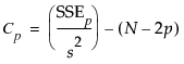
where s2 is the MSE for the full model and SSEp is the sum-of-squares error for a model with p variables, including the intercept. Note that p is the number of x-variables+1. If Cp is graphed with p, Mallows (1973) recommends choosing the model where Cp first approaches p.
p
Number of parameters in the model, including the intercept.
AICc
Corrected Akaike’s Information Criterion. For more details, see “Likelihood, AICc, and BIC” in the “Statistical Details” appendix.
BIC
Bayesian Information Criterion. For more details, see “Likelihood, AICc, and BIC” in the “Statistical Details” appendix.
Forward Selection Example
In forward selection, terms are entered into the model and most significant terms are added until all of the terms are significant.
1. Complete the steps in “Example Using Stepwise Regression”.
Notice that the default selection for Direction is Forward.
2. Click Step.
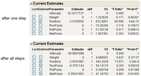
From the top figure in Figure 5.4, you can see that after one step, the most significant term, Runtime, is entered into the model.
3. Click Go.
The bottom figure in Figure 5.4 shows that all of the terms have been added, except RstPulse and Weight.
Figure 5.4 Current Estimates Table for Forward Selection
Backward Selection Example
In backward selection, all terms are entered into the model and then the least significant terms are removed until all of the remaining terms are significant.
1. Complete the steps in “Example Using Stepwise Regression”.
2. Click Enter All.
Figure 5.5 All Effects Entered Into the Model
3. For Direction, select Backward.
4. Click Step two times.
The first backward step removes RstPulse and the second backward step removes Weight.
Figure 5.6 Current Estimates with Terms Removed and Step History Table
The Current Estimates and Step History tables shown in Figure 5.6 summarize the backward stepwise selection process. Note the BIC value of 156.362 for the third step in the Step History table. If you click Step again to remove another parameter from the model, the BIC value increases to 159.984. For this reason, you choose the step 3 model. This is also the model that the Go button produces.
Current Estimates Report
Use the Current Estimates report to enter, remove, and lock in model effects. (The intercept is permanently locked into the model.)
Figure 5.7 Current Estimates Table
Lock
Locks a term in or out of the model. A checked term cannot be entered or removed from the model.
Entered
Indicates whether a term is currently in the model. You can click a term’s check box to manually bring an effect in or out of the model.
Parameter
Lists effect names.
Estimate
Current parameter estimate (zero if the effect is not currently in the model).
nDF
Number of degrees of freedom for a term. A term has more than one degree of freedom if its entry into a model also forces other terms into the model.
SS
Reduction in the error (residual) sum of squares (SS) if the term is entered into the model or the increase in the error SS if the term is removed from the model. If a term is restricted in some fashion, it could have a reported SS of zero.
“F Ratio”
Traditional test statistic to test that the term effect is zero. It is the square of a t-ratio. It is in quotation marks because it does not have an F-distribution for testing the term because the model was selected as it was fit.
“Prob>F”
Significance level associated with the F statistic. Like the “F Ratio,” it is in quotation marks because it is not to be trusted as a real significance probability.
R
Multiple correlation with the other effects in the model.
Note: Appears only if you right-click in the report and select Columns > R.
Step History Report
As each step is taken, the Step History report records the effect of adding a term to the model. For example, the Step History report for the Fitness.jmp example shows the order in which the terms entered the model and shows the statistics for each model. See “Example Using Stepwise Regression”.
Use the radio buttons on the right to choose a model.
Figure 5.8 Step History Report
Models with Crossed, Interaction, or Polynomial Terms
Some models, especially those associated with experimental designs, involve interaction terms. For continuous factors, these are products of the columns representing the effects. For nominal and ordinal factors, interactions are defined by model terms that involve products of terms representing the categorical levels.
When there are interaction terms, you often want to impose a restriction on the model selection process so that lower-order components of higher-order effects are included in the model. This is suggested by the principle of Effect Heredity. See the Starting Out chapter in the Design of Experiments Guide. For example, if a two-way interaction is included in a model, its component main effects (precedents) should be included as well.
Example of the Combine Rule
1. Select Help > Sample Data Library and open Reactor.jmp.
2. Select Analyze > Fit Model.
3. Select Y and click Y.
4. In the Degree box, type 2.
5. Select F, Ct, A, T, and Cn and click Macros > Factorial to Degree.
6. For Personality, select Stepwise.
7. Click Run.
Figure 5.9 Initial Current Estimates Report Using Combine Rule

The model in Figure 5.9 contains all terms for up to two-factor interactions for the five continuous factors. The Combine, Restrict, and Whole Effects rules described in “Rules” enable you to control entry of interaction terms.
The Combine rule determines the entry of interaction terms based on two tests. See “Combine”. You can determine which of the two tests was used for the p-value based on the degrees of freedom, nDF. For example, the interaction term F*A has an nDF value of 3. This means that F*A is grouped with its precedent terms F and A, and is considered for entry based on the 3 degree of freedom joint F test. In contrast, the interaction term Ct*T has an nDF value of 1. This means that Ct*T is considered for entry based on the 1 degree of freedom F test that tests the significance of Ct*T after its precedent terms, Ct and T, are already included in the model.Click Step once to see that Ct is entered by itself.
8. Click Step again to see that Ct*T is entered, along with T (Ct is already in the model).
Figure 5.10 Current Estimates Report Using Combine Rule, One Step
When there are significant interaction terms, several terms can enter at the same step. If the Step button is clicked twice, Ct*T is entered along with its two contained effects Ct and T. However, a step back is not symmetric because a crossed term can be removed without removing its two component terms. Notice that Ct and T now each have 2 degrees of freedom. This is because if Stepwise removes Ct or T, it must also remove Ct*T. If you change the Direction to Backward and click Step, Ct*T is removed and the degrees of freedom for Ct and T change to 1.
Models with Nominal and Ordinal Effects
Traditionally, stepwise regression has not addressed the situation where there are categorical effects in the model. Note the following:
• When a regression model contains nominal or ordinal effects, those effects are represented by sets of indicator columns.
• When a categorical effect has only two levels, that effect is represented by a single column.
• When a categorical effect has k levels, where k > 2, then it must be represented by k-1 columns.
The convention in JMP for standard platforms is to represent nominal variables by terms whose parameter estimates average to zero across all the levels.
In the Stepwise platform, categorical variables (nominal and ordinal) are coded in a hierarchical fashion. This differs from coding in other least squares fitting platforms. In hierarchical coding, the levels of the categorical variable are successively split into groups of levels that most separate the means of the response. The splitting process achieves the goal of representing a k-level categorical variable by k - 1 terms.
Note: In hierarchical coding, the initial terms that are constructed represent the groups responsible for the greatest separation. The advantage of this coding scheme is that these informative terms have the potential to enter the model early.
Construction of Hierarchical Terms
Hierarchical terms are constructed using a tree structure that is analogous to a Partition analysis. However, the criterion that is maximized is the sum of squares between groups (SSB).
For a nominal variable with k levels, the k levels are split into two groups of levels that have maximum SSB. Call these two groups of levels A1 and A2, where A1 has the smaller mean and A2 has the larger mean. The two groups of levels in A1 and A2 are used to define an indicator variable with values of 1 for the levels in A1 and -1 for the levels in A2. This variable is the first hierarchical term for the nominal variable.
For the levels within each of the initial two groups A1 and A2, the split into two groups of levels with the maximum SSB is identified. Suppose that the groups of levels with maximum SSB are among the levels in A1. Call the two groups B1 and B2, where A1 has the smaller mean and A2 has the larger mean. The two groups of levels in B1 and B2 are used to define a hierarchical variable with values of 1 for the levels in B1, -1 for the levels in B2, and 0 for the levels in A2. To construct the next variable, splits of the levels in B1, B2, and A2 are considered. The split that maximizes SSB defines the next hierarchical variable. The process continues until k-1 hierarchical terms are constructed.
For an ordinal variable, the groups of levels considered in splitting contain only levels that are contiguous in the ordering. This ensures that the constructed terms respect the level ordering.
Rules and Hierarchical Terms
When you use the Combine rule or the Restrict rule, a term cannot enter the model unless all the terms above it in the hierarchy have been entered. When you use the Whole Effects rule and enter a term for a categorical variable, all of its associated terms are entered. For an example, see “Construction of Hierarchical Terms in Example”.
Example of a Model with a Nominal Term
This example uses data on movies that were released in 2011. You are particularly interested in the World Gross values, which represent the gross receipts. Your potential predictors are Rotten Tomatoes Score, Audience Score, and Genre. The two score variables are continuous, but Genre is nominal. Before you attempt to reduce your model using Stepwise, you want to explore the variables of interest.
1. Select Help > Sample Data Library and open Hollywood Movies.jmp.
2. Select Analyze > Distribution.
3. Select Genre and click Y, Columns.
4. Click OK.
Figure 5.11 Distribution of Genre
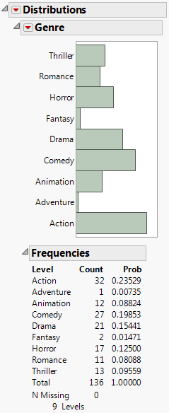
Note that Genre has nine levels, and so would be represented by eight model terms. Further data exploration will reveal that, because of missing data, only eight levels are considered by Stepwise.
5. In the data table’s Columns panel, select the columns of interest: Rotten Tomatoes Score, Audience Score, Genre, and World Gross.
6. Selects Cols > Modeling Utilities > Explore Missing Values.
Figure 5.12 Missing Columns Report
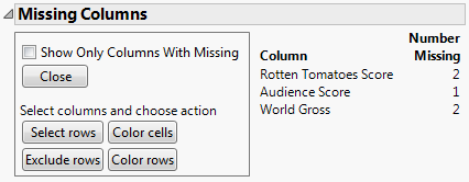
Note that Rotten Tomatoes Score is missing in 2 rows, Audience Score is missing in 1 row, and World Gross is missing in 2 rows.
7. In the Missing Columns report, select the three columns listed under Column.
8. Click Select Rows.
In the data table’s Rows panel, you can see that three rows are selected. Because these three rows contain missing data on the predictors or response, they will be automatically excluded from the Stepwise analysis. Note that row 134 is the only entry in the Adventure category, which means that category will be entirely removed from the analysis. For the purposes of the Stepwise analysis, it follows that Genre has only eight categories. Now that you have seen the effect of the missing data, you will conduct the Stepwise analysis.
9. Select Analyze > Fit Model.
10. Select Rotten Tomatoes Score, Audience Score, and Genre and click Add.
If you fit a standard least squares model to World Gross using Rotten Tomatoes Score, Audience Score, and Genre as predictors, the residuals are highly heteroskedastic. (This is typical of financial data.) Use a log transformation to better satisfy the regression assumption of equal variance.
11. Right-click on World Gross in the Select Columns list and select Transform > Log.
The transformed variable Log[World Gross] appears at the bottom of the Select Columns list.
12. Select Log[World Gross] and click Y.
13. Select Stepwise from the Personality list.
14. Click Run.
Figure 5.13 Current Estimates Table Showing List of Model Terms
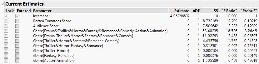
In the Current Estimates table, note that Genre is represented by 7 terms. You will construct a model using two of these to see how these terms are defined.
15. Check the boxes under Entered next to the first two terms for Genre:
‒ Genre{Drama&Thriller&Horror&Fantasy&Romance&Comedy-Action&Animation}
‒ Genre{Drama-Thriller&Horror&Fantasy&Romance&Comedy}
16. Click Make Model.
Notice that the two terms are added to the Model Effects list in the Model Specification window. Also notice that two columns representing these terms have been added to the data table. These columns are discussed in the next section.
Construction of Hierarchical Terms in Example
Recall that because of missing values, Genre is a nominal variable with eight levels. In the Current Estimates table, Genre is represented by seven terms. This is appropriate, because Genre has eight levels. The first two terms that represent Genre are described below. Subsequent terms are defined in a similar fashion.
First Term
The first term that appears is Genre{Drama&Thriller&Horror&Fantasy&Romance&Comedy-Action&Animation}. This variable has the form Genre{A1 - A2}, where A1 and A2 are separated by a minus sign. The notation indicates that the maximum separation in terms of sum of squares between groups occurs between the following two sets of levels:
• Drama, Thriller, Horror, Fantasy, Romance, and Comedy (represented by A1)
• Action and Animation (represented by A2)
If you include the term Genre{Drama&Thriller&Horror&Fantasy&Romance&Comedy-Action&Animation} in a model, a column representing that term is added to the data table. In the example, you saved this column to the data table. The column shows the following values:
• 1 for Drama, Thriller, Horror, Fantasy, Romance, and Comedy
• -1 for Action and Animation
Second Term
The second term that appears is Genre{Drama-Thriller&Horror&Fantasy&Romance&Comedy}. This set of levels is entirely contained in the first split for the first term (A1). The notation contrasts the levels:
• Drama,
• Thriller, Horror, Fantasy, Romance, and Comedy
Among all the splits of the levels of Drama, Thriller, Horror, Fantasy, Romance, and Comedy (A1) and of the levels of Action and Animation (A2), the algorithm determines that this split has the largest SSB.
If you include this term in a model, a column representing that term is added to the data table. In the example, you saved this column to the data table. The column shows the following values:
• 1 for Drama
• -1 for Thriller, Horror, Fantasy, Romance, and Comedy
• 0 for Action and Animation
Hierarchy of Terms
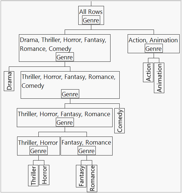
The splitting of terms continues, based on the sum of squares between groups criterion. The hierarchy that leads to the definition of the terms is illustrated in Figure 5.14.
Figure 5.14 Tree Showing Splits Used in Hierarchical Coding
Rules
When you use the Combine rule or the Restrict rule, a term cannot enter the model unless all the terms above it in the hierarchy have been entered. For example, if you enter Genre{Action-Animation}, then JMP will enter Genre{Drama&Thriller&Horror&Fantasy&Romance&Comedy-Action&Animation} as well.
When you use the Whole Effects rule and enter any one of the Genre terms, all of the Genre terms are entered.
Example of the Restrict Rule for Hierarchical Terms
If you have a model with nominal or ordinal terms, when you make or run the model, columns containing the hierarchical terms involved in the model are added to the data table. The model itself appears in a new Fit Model window. This example further illustrates how Stepwise constructs a model with hierarchical effects.
A simple model examines at the cost per ounce ($/oz) of hot dogs as a function of the Type of hot dog (Meat, Beef, Poultry) and the Size of the hot dog (Jumbo, Regular, Hors d’oeuvre).
1. Select Help > Sample Data Library and open Hot Dogs2.jmp.
2. Select Analyze > Fit Model.
3. Select $/oz and click Y.
4. Select Type and Size and click Add.
5. For Personality, select Stepwise.
6. Click Run.
7. For Stopping Rule, select P-value Threshold.
8. For Rules, select Restrict.
Figure 5.15 Stepwise Control Panel with P-value Threshold and Restrict Rule
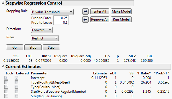
Notice that when you change from the default Rule of Combine to Restrict, the F Ratio and Prob > F values for two terms are shown as missing. These are the terms Type{Poultry-Meat} and Size{Regular-Jumbo}. This is because these two terms cannot enter the model until their precedent terms enter.
9. Click Step.
The term Type{Poultry&Meat-Beef} enters the model. This term has the smallest Prob>F value, and that value falls below the Prob to Enter threshold of 0.25.
Figure 5.16 Stepwise Control Panel with One Term Entered
The the F Ratio and Prob > F values for the term Type{Poultry-Meat} appear. Since its precedent term has entered the model, Type{Poultry-Meat} is now allowed to enter.
10. Click Step.
Since Type{Poultry-Meat} has the smallest Prob>F value among the remaining terms, and that value is below the Prob to Enter threshold, it is the next term to enter the model.
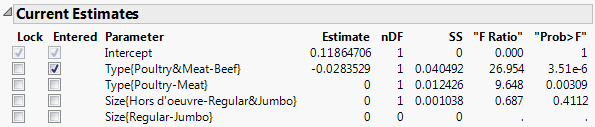
11. Click Step.
The term Size{Hors d'oeuvre-Regular&Jumbo} enters the model, since its Prob>F value is 0.1577. Because its precedent term is now in the model, the term Size{Regular-Jumbo} is allowed to enter the model and its Prob>F value appears.
However, the Prob>F value for the term Size{Regular-Jumbo} is 0.7566, which exceeds the Prob to Enter value of 0.25. For this reason, if you click Step again, it is not entered into the model.
Figure 5.17 Current Estimates Report for the Final Model
Tip: Use the Go button to run the entire stepwise process automatically. To see this in action, click Remove All. Then click Go.
12. Click Make Model.
After you click Make Model, a Fit Model launch window appears, containing only the three model effects that were selected in the stepwise process. In the data table, columns are added that define the three hierarchical effects entered into the model.
Performing Binary and Ordinal Logistic Stepwise Regression
The Stepwise personality of Fit Model performs ordinal logistic stepwise regression when the response is ordinal or nominal. Nominal responses are treated as ordinal responses in the logistic stepwise regression fitting procedure. To run a logistic stepwise regression, specify an ordinal or nominal response, add terms to the model as usual, and choose Stepwise from the Personality menu.
The Stepwise reports for a logistic model are similar to those provided when the response is continuous. The following elements are specific to logistic regression results:
• When the response is categorical, the overall fit of the model is given by its negative log-likelihood (-LogLikelihood). This value is calculated based on the full iterative maximum likelihood fit.
• The Current Estimates report shows chi-square statistics (Wald/Score ChiSq) and their p-values (Sig Prob). The test statistic column shows score statistics for parameters that are not in the current model and shows Wald statistics for parameters that are in the current model. The regression estimates (Estimate) are based on the full iterative maximum likelihood fit.
• The Step History report shows the L-R ChiSquare. This value is the test statistic for the likelihood ratio test of the hypothesis that the corresponding regression parameter is zero, given the other terms in the model. The Sig Prob is the p-value for this test.
Note: If the response is nominal, you can fit the current model using the Nominal Logistic personality of Fit Model by clicking the Make Model button. In the Fit Model launch window that appears, click Run.
Example Using Logistic Stepwise Regression
1. Select Help > Sample Data Library and open Fitness.jmp.
2. Select Analyze > Fit Model.
3. Select Sex and click Y.
4. Select Weight, Runtime, RunPulse, RstPulse, and MaxPulse and click Add.
5. For Personality, select Stepwise.
6. Click Run.
7. Click Go.
Figure 5.18 Logistic Stepwise Report
The two variables Weight and Runtime are entered into the model based on the Stopping Rule.
8. Click Make Model.
Figure 5.19 Model Specification Window for Reduced Model
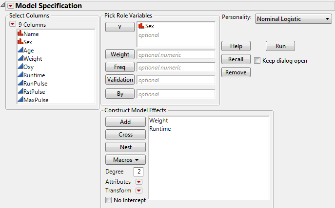
A model specification window opens containing the two variables as model effects. Note that the Personality is Nominal Logistic. If the response had been ordinal, the Personality would be Ordinal Logistic.
The All Possible Models Option
Use the All Possible Models option to investigate all models that can be constructed using your predictors. This option is accessed from the red triangle menu next to Stepwise.
Note the following:
• This option is not practical for large problems, when the number of models is greater than 5 million.
• Categorical predictors are represented by indicator variables. See “Models with Nominal and Ordinal Effects”.
The following options restrict the number of models that appear:
Maximum number of terms in a model
Enter a value for the maximum number of terms in a model.
Number of best models to see
Enter the maximum number of models of each size to display. The best models according to RSquare value appear.
Restrict to models where interactions imply lower order effects (Heredity Restriction)
Shows only models that contain all lower-order effects when a higher-order effect is included. These models satisfy strong effect heredity. This option is useful when your predictors include interaction or polynomial terms.
Example Using the All Possible Models Option
1. Select Help > Sample Data Library and open Fitness.jmp.
2. Select Analyze > Fit Model.
3. Select Oxy and click Y.
4. Select Runtime, RunPulse, RstPulse, and MaxPulse and click Add.
5. For Personality, select Stepwise.
6. Click Run.
7. From the red triangle menu next to Stepwise, select All Possible Models.
8. Enter 3 for the maximum number of terms, and enter 5 for the number of best models.
Figure 5.20 All Possible Models Popup Dialog
9. Click OK.
All possible models (up to three terms in a model) are fit.
Figure 5.21 All Possible Models Report
The models are listed in increasing order of the number of parameters that they contain. The model with the highest R2 for each number of parameters is highlighted. The radio button column at the right of the table enables you to select one model at a time and check the results.
Note: The recommended criterion for selecting a model is to choose the one corresponding to the smallest BIC or AICc value. Some analysts also want to see the Cp statistic. Mallow’s Cp statistic is computed, but initially hidden in the table. To make it visible, right-click in the table and select Columns > Cp.
The Model Averaging Option
The model averaging technique enables you to average the fits for a number of models, instead of picking a single best model. The result is a model with excellent prediction capability. This feature is particularly useful for new and unfamiliar models that you do not want to overfit. When many terms are selected into a model, the fit tends to inflate the estimates. Model averaging tends to shrink the estimates on the weaker terms, yielding better predictions. The models are averaged with respect to the AICc weight, calculated as follows:
AICcBest is the smallest AICc value among the fitted models. The AICc Weights are then sorted in decreasing order. The AICc weights cumulating to less than one minus the cutoff of the total AICc weight are set to zero, allowing the very weak terms to have true zero coefficients instead of extremely small coefficient estimates.
Example Using the Model Averaging Option
1. Select Help > Sample Data Library and open Fitness.jmp.
2. Select Analyze > Fit Model.
3. Select Oxy and click Y.
4. Select Runtime, RunPulse, RstPulse, and MaxPulse and click Add.
5. For Personality, select Stepwise.
6. Click Run.
7. From the red triangle menu next to Stepwise, select Model Averaging.
8. Enter 3 for the maximum number of terms, and keep 0.95 for the weight cutoff.
Figure 5.22 Model Averaging Window
9. Click OK.
Figure 5.23 Model Averaging Report
In the Model Averaging report, average estimates and standard errors appear for each parameter. The standard errors shown reflect the bias of the estimates toward zero.
10. Click Save Prediction Formula to save the prediction formula in the original data table.
Using Validation
In JMP, you can perform cross-validation by selecting the K-Fold Crossvalidation option from the Stepwise Fit red triangle menu.
In JMP Pro, you can specify a Validation column in the Fit Model window. A validation column must have a numeric data type and should contain at least two distinct values.
• If the column contains two values, the smaller value defines the training set and the larger value defines the validation set.
• If the column contains three values, the values define the training, validation, and test sets in order of increasing size.
• If the column contains four or more distinct values and the response is continuous, these values define folds for k-fold validation.
Validation Set with Two or Three Values
If the response is continuous, the following statistics appear in the Stepwise Regression Control panel:
• RSquare Validation (also shown in the Step History report)
• RMSE Validation
• RSquare Test (if there is a test set)
• RMSE Test (if there is a test set)
If the response is binary nominal or ordinal, the following statistics appear in the Stepwise Regression Control panel:
• RSquare Validation (also shown in the Step History report)
• Avg Log Error Validation
• RSquare Test (if there is a test set)
• Avg Log Error Test (if there is a test set)
Max Validation RSquare
If you specify a validation column with two or three values in the Fit Model window, the Stopping Rule defaults to Max Validation RSquare. This rule attempts to find a model that maximizes the RSquare statistic for the validation set. The rule can be applied with the Direction set to Forward or Backward.
Note: Max Validation RSquare considers only the models defined by p-value entry (Forward direction) or removal (Backward direction). It does not consider all possible models.
You can use the Step button to enter terms one-by-one in the Forward direction or to remove them one-by one in the Backward direction. At any point, you can select a model by clicking the button to the right of RSquare Validation in the Step History report. The selection of model terms is updated in the Current Estimates report. This is the model that is used once you click Make Model or Run Model.
Forward Direction
In the Forward direction, Stepwise constructs successive models by adding terms based on the next smallest p-value.
If you click Go rather than Step, the process of entering terms proceeds automatically. Among the fitted models, the model that is considered best is listed last. This model is obtained by overlooking local dips in RSquare Validation. Specifically, it is the model with the largest RSquare Validation that can be followed by as many as ten models with lower RSquare Validation values. This model is designated by the terms Best in the Parameter column and Specific in the Action column. The button to the right of RSquare Validation selects this Best model, though you are free to change this selection.
Backward Direction
In the Backward direction, Stepwise constructs successive models by removing terms based on the next largest p-value.
To use the Backward direction, you must first click Enter All to enter all of the terms into the model. The Backward direction behaves in a similar fashion to the Forward direction. If you click Go rather than Step, the process of removing terms proceeds automatically. The model designated as Best is the one with the largest RSquare Validation that can be followed by as many as ten models with lower RSquare Validation values.
Validation and Test Set Statistic Definitions
RSquare Validation and RMSE Validation are defined in this section. RSquare Test and RMSE Test are computed for the test set in a completely analogous fashion.
Continuous Response
RSquare Validation
An RSquare measure for the validation set computed as follows:
‒ For each observation in the validation set, compute the prediction error. This is the difference between the actual response and the response predicted by the training set model.
‒ Square and sum the prediction errors to obtain SSEValidation.
‒ Square and sum the differences between the actual responses in the validation set and their mean. This is the SSTValidation.
‒ RSquare Validation is:
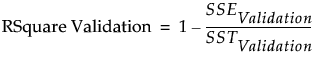
Note: It is possible for RSquare Validation to be negative.
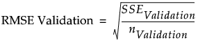
RMSE Validation
The square root of the mean squared prediction error for the validation set. This is computed as follows:
‒ For each observation in the validation set, compute the prediction error. This is the difference between the actual response and the response predicted by the training set model.
‒ Square and sum the prediction errors to obtain the SSEValidation.
‒ Denote the number of observations in the validation set by nValidation.
‒ RMSE Validation is:
Note: In the Fit Least Squares Crossvalidation report, the entries in the RASE (Root Average Squared Error) column for the Validation Set and Test Set are the RMSE Validation and RMSE Test values computed in the Stepwise report. See “RASE”.
Binary Nominal or Ordinal Response
RSquare Validation
An Entropy RSquare measure (also known as McFadden’s R2) for the validation set computed as follows:
‒ A model is fit using the training set.
‒ Predicted probabilities are obtained for all observations.
‒ Using the predicted probabilities based on the training set model, the likelihood for the model is computed for observations in the validation set. Call this quantity Likelihood_FullValidation.
‒ Using the data in the validation set, the likelihood of the reduced model (no predictors) is computed. Call this quantity Likelihood_ReducedValidation.
‒ RSquare Validation is:
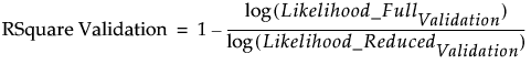
Note: It is possible for RSquare Validation to be negative.
Avg Log Error Validation
The average log error for the validation set is computed as follows:
‒ For each observation in the validation set, compute the log of its predicted probability as determined by the model based on the training set.
‒ Sum these logs, divide by the number of observations in the validation set, and take the negative of the resulting value.
Tip: Smaller values of Avg Log Error Validation are desirable.
K-Fold Cross Validation
K-fold cross validation randomly divides the data into k subsets. In turn, each of the k sets is used as a validation set while the remaining data are used as a training set to fit the model. In total, k models are fit and k validation statistics are obtained. The model giving the best validation statistic is chosen as the final model. This method is useful for small data sets, because it makes efficient use of limited amounts of data.
Note: K-fold cross validation is only available for continuous responses.
In JMP, select K-Fold Crossvalidation from the red triangle options for Stepwise Fit.
In JMP Pro, you can access k-fold cross validation in two ways:
• From the red triangle options for Stepwise Fit, select K-Fold Crossvalidation.
• Specify a validation column with four or more distinct values.
RSquare K-Fold Statistic
If you conduct k-fold cross validation, the RSquare K-Fold statistic appears to the right of the other statistics in the Stepwise Regression Control panel. RSquare K-Fold is the average of the RSquare Validation values for the k folds.
Max K-Fold RSquare
When you use k-fold cross validation, the Stopping Rule defaults to Max K-Fold RSquare. This rule attempts to maximize the RSquare K-Fold statistic.
Note: Max K-Fold RSquare considers only the models defined by p-value entry (Forward direction) or removal (Backward direction). It does not consider all possible models.
The Max K-Fold RSquare stopping rule behaves in a fashion similar to the Max Validation RSquare stopping rule. See “Max Validation RSquare”. Replace references to RSquare Validation with RSquare K-Fold.
..................Content has been hidden....................
You can't read the all page of ebook, please click here login for view all page.