
Example of a Multiple Response Model
This example uses the Golf Balls.jmp sample data table (McClave and Dietrich, 1988). The data are a comparison of distances traveled and a measure of durability for three brands of golf balls. A robotic golfer hit a random sample of ten balls for each brand in a random sequence. The hypothesis to test is that distance and durability are the same for the three golf ball brands.
1. Select Help > Sample Data Library and open Golf Balls.jmp.
2. Select Analyze > Fit Model.
3. Select Distance and Durability and click Y.
4. Select Brand and click Add.
5. For Personality, select Manova.
Figure 9.1 Manova Setup
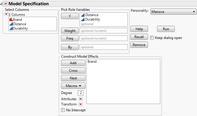
6. Click Run.
Figure 9.2 Manova Report Window

The initial results might not be very interesting in themselves, because no response design has been specified yet. After you specify a response design, the multivariate platform displays tables of multivariate estimates and tests. For details about specifying a response design, see “Response Specification”.
The Manova Report
The Manova report window contains the following elements:
Manova Fit red triangle menu
Contains save options. See “The Manova Fit Options”.
Response Specification
Enables you to specify the response designs for various tests. See “Response Specification”.
Parameter Estimates
Contains the parameter estimates for each response variable (without details like standard errors or t-tests). There is a column for each response variable.
Least Squares Means
Reports the overall least squares means of all of the response columns, least squares means of each nominal level, and least squares means plots of the means.
Partial Correlation
Shows the covariance matrix and the partial correlation matrix of residuals from the initial fit, adjusted for the X effects.
Overall E&H Matrices
Shows the E and H matrices:
‒ The elements of the E matrix are the cross products of the residuals.
‒ The H matrices correspond to hypothesis sums of squares and cross products.
There is an H matrix for the whole model and for each effect in the model. Diagonal elements of the E and H matrices correspond to the hypothesis (numerator) and error (denominator) sum of squares for the univariate F tests. New E and H matrices for any given response design are formed from these initial matrices, and the multivariate test statistics are computed from them.
The Manova Fit Options
The following Manova Fit options are available:
Save Discrim
Performs a discriminant analysis and saves the results to the data table. For more details, see “Discriminant Analysis”.
Save Predicted
Saves the predicted responses to the data table.
Save Residuals
Saves the residuals to the data table.
Model Dialog
Shows the completed launch window for the current analysis.
See the JMP Reports chapter in the Using JMP book for more information about the following options:
Local Data Filter
Shows or hides the local data filter that enables you to filter the data used in a specific report.
Redo
Contains options that enable you to repeat or relaunch the analysis. In platforms that support the feature, the Automatic Recalc option immediately reflects the changes that you make to the data table in the corresponding report window.
Save Script
Contains options that enable you to save a script that reproduces the report to several destinations.
Save By-Group Script
Contains options that enable you to save a script that reproduces the platform report for all levels of a By variable to several destinations. Available only when a By variable is specified in the launch window.
Response Specification
Specify the response designs for various tests using the Response Specification panel.
Figure 9.3 Response Specification Panel
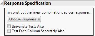
Choose Response
Provides choices for the M matrix. See “Choose Response Options”.
Univariate Tests Also
Obtains adjusted and unadjusted univariate repeated measures tests and multivariate tests. Use in repeated measures models.
Test Each Column Separately Also
Obtains univariate ANOVA tests and multivariate tests on each response.
The following buttons only appear after you have chosen a response option:
Run
Performs the analysis and shows the multivariate estimates and tests. See “Multivariate Tests”.
Help
Shows the help for the Response Specification panel.
Orthogonalize
Orthonormalizes the matrix. Orthonormalization is done after the column contrasts (sum to zero) for all response types except Sum.
Delete Last Column
Reduces the dimensionality of the transformation.
Choose Response Options
The response design forms the M matrix. The columns of an M matrix define a set of transformation variables for the multivariate analysis. The Choose Response button contains the options for the M matrix.
Repeated Measures
Constructs and runs both Sum and Contrast responses.
Sum
Sum of the responses that gives a single value.
Identity
Uses each separate response, the identity matrix.
Contrast
Compares each response and the first response.
Polynomial
Constructs a matrix of orthogonal polynomials.
Helmert
Compares each response with the combined responses listed below it.
Profile
Compares each response with the following response.
Mean
Compares each response with the mean of the others.
Compound
Creates and runs several response functions that are appropriate if the responses are compounded from two effects.
Custom
Uses any custom M matrix that you enter.
The most typical response designs are Repeated Measures and Identity for multivariate regression. There is little difference in the tests given by the Contrast, Helmert, Profile, and Mean options, since they span the same space. However, the tests and details in the Least Squares means and Parameter Estimates tables for them show correspondingly different highlights.
The Repeated Measures and the Compound options display dialogs to specify response effect names. They then fit several response functions without waiting for further user input. Otherwise, selections expand the control panel and give you more opportunities to refine the specification.
Custom Test Option
Set up custom tests of effect levels using the Custom Test option.
Note: For instructions on how to create custom tests, see “Custom Test” in the “Standard Least Squares Report and Options” chapter.
The menu icon beside each effect name gives you the commands shown here, to request additional information about the multivariate fit:
Test Details
Displays the eigenvalues and eigenvectors of the  matrix used to construct multivariate test statistics. See “Test Details”.
Centroid Plot
Plots the centroids (multivariate least squares means) on the first two canonical variables formed from the test space. See “Centroid Plot”.
Save Canonical Scores
Saves variables called Canon[1], Canon[2], and so on, as columns in the current data table. These columns have both the values and their formulas. For an example, see “Save Canonical Scores”. For technical details, see “Canonical Details”.
Contrast
Performs the statistical contrasts of treatment levels that you specify in the contrasts dialog.
Note: The Contrast command is the same as for regression with a single response. See the “LSMeans Contrast” in the “Standard Least Squares Report and Options” chapter, for a description and examples of the LSMeans Contrast commands.
Test Details
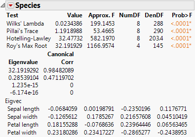
The Test Details report gives canonical details about the test for the whole model or the specified effect.
Eigenvalue
Lists the eigenvalues of the  matrix used in computing the multivariate test statistics.
Canonical Corr
Lists the canonical correlations associated with each eigenvalue. This is the canonical correlation of the transformed responses with the effects, corrected for all other effects in the model.
Eigvec
Lists the eigenvectors of the  matrix, or equivalently of
  .
.
Example of Test Details
1. Select Help > Sample Data Library and open Iris.jmp.
The Iris data (Mardia, Kent, and Bibby 1979) have three levels of Species named Virginica, Setosa, and Versicolor. There are four measures (Petal length, Petal width, Sepal length, and Sepal width) taken on each sample.
2. Select Analyze > Fit Model.
3. Select Petal length, Petal width, Sepal length, and Sepal width and click Y.
4. Select Species and click Add.
5. For Personality, select Manova.
6. Click Run.
7. Click on the Choose Response button and select Identity.
8. Click Run.
9. From the red triangle menu next to Species, select Test Details.
The eigenvalues, eigenvectors, and canonical correlations appear. See Figure 9.4.
Figure 9.4 Test Details
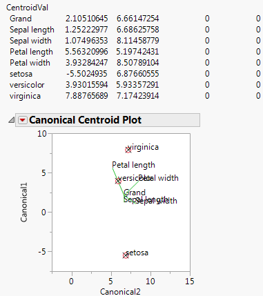
Centroid Plot
The Centroid Plot command (accessed from the red triangle next to Species) plots the centroids (multivariate least squares means) on the first two canonical variables formed from the test space, as in Figure 9.5. The first canonical axis is the vertical axis so that if the test space is only one dimensional the centroids align on a vertical axis. The centroid points appear with a circle corresponding to the 95% confidence region (Mardia, Kent, and Bibby, 1979). When centroid plots are created under effect tests, circles corresponding to the effect being tested appear in red. Other circles appear blue. Biplot rays show the directions of the original response variables in the test space. See “Details for Centroid Plot”.
Click the Centroid Val disclosure icon to show additional information, shown in Figure 9.5.
The first canonical axis with an eigenvalue accounts for much more separation than does the second axis. The means are well separated (discriminated), with the first group farther apart than the other two. The first canonical variable seems to load the petal length variables against the petal width variables. Relationships among groups of variables can be verified with Biplot Rays and the associated eigenvectors.
Figure 9.5 Centroid Plot and Centroid Values
Save Canonical Scores
Saves columns called Canon[i] to the data table, where i refers to the ith canonical score for the Y variables. The canonical scores are computed based on the  matrix used to construct the multivariate test statistic. Canonical scores are saved for eigenvectors corresponding to nonzero eigenvalues.
Canonical Correlation
Canonical correlation analysis is not a specific command, but it can be done by a sequence of commands in the multivariate fitting platform, as follows:
2. From the red triangle menu next to Whole Model, select Test Details.
3. From the red triangle menu next to Whole Model, select Save Canonical Scores.
The details list the canonical correlations (Canonical Corr) next to the eigenvalues. The saved variables are called Canon[1], Canon[2], and so on. These columns contain both the values and their formulas.
To obtain the canonical variables for the X side, repeat the same steps, but interchange the X and Y variables. If you already have the columns Canon[n] appended to the data table, the new columns are called Canon[n] 2 (or another number) that makes the name unique.
For another example, proceed as follows:
1. Select Help > Sample Data Library and open Exercise.jmp.
2. Select Analyze > Fit Model.
3. Select chins, situps, and jumps and click Y.
4. Select weight, waist, and pulse and click Add.
5. For Personality, select Manova.
6. Click Run.
7. Click on the Choose Response button and select Identity.
8. Click Run.
9. From the red triangle menu next to Whole Model, select Test Details.
10. From the red triangle menu next to Whole Model, select Save Canonical Scores.
Figure 9.6 Canonical Correlations

The output canonical variables use the eigenvectors shown as the linear combination of the Y variables. For example, the formula for canon[1] is as follows:
0.02503681*chins + 0.00637953*situps + -0.0052909*jumps
This canonical analysis does not produce a standardized variable with mean 0 and standard deviation 1, but it is easy to define a new standardized variable with the calculator that has these features.
Multivariate Tests
Example Choosing a Response
2. Click on the Choose Response button and select Identity.
3. Click Run.
Figure 9.7 Multivariate Test Reports
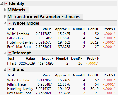
The M Matrix report gives the response design that you specified. The M-transformed Parameter Estimates report gives the original parameter estimates matrix multiplied by the transpose of the M matrix.
Note: Initially in this chapter, the matrix names E and H refer to the error and hypothesis cross products. After specification of a response design, E and H refer to those matrices transformed by the response design, which are actually M´EM and M´HM.
The Extended Multivariate Report
In multivariate fits, the sums of squares due to hypothesis and error are matrices of squares and cross products instead of single numbers. And there are lots of ways to measure how large a value the matrix for the hypothesis sums of squares and cross products (called H or SSCP) is compared to that matrix for the residual (called E). JMP reports the four multivariate tests that are commonly described in the literature. If you are looking for a test at an exact significance level, you may need to go hunting for tables in reference books. Fortunately, all four tests can be transformed into an approximate F test. If the response design yields a single value, or if the hypothesis is a single degree of freedom, the multivariate tests are equivalent and yield the same exact F test. JMP labels the test Exact F; otherwise, JMP labels it Approx. F.
In the golf balls example, there is only one effect so the Whole Model test and the test for Brand are the same, which show the four multivariate tests with approximate F tests. There is only a single intercept with two DF (one for each response), so the F test for it is exact and is labeled Exact F.
The red triangle menus on the Whole Model, Intercept, and Brand reports contain options to generate additional information, which includes eigenvalues, canonical correlations, a list of centroid values, a centroid plot, and a Save command that lets you save canonical variates.
The effect (Brand in this example) popup menu also includes the option to specify contrasts.
The custom test and contrast features are the same as those for regression with a single response. See the “Standard Least Squares Report and Options” chapter.
To see formulas for the MANOVA table tests, see “Multivariate Tests”.
The extended Multivariate Report contains the following columns:
Test
Labels each statistical test in the table. If the number of response function values (columns specified in the M matrix) is 1 or if an effect has only one degree of freedom per response function, the exact F test is presented. Otherwise, the standard four multivariate test statistics are given with approximate F tests: Wilks’ Lambda (Λ), Pillai’s Trace, the Hotelling-Lawley Trace, and Roy’s Maximum Root.
Value
Value of each multivariate statistical test in the report.
Approx. F (or Exact F)
F-values corresponding to the multivariate tests. If the response design yields a single value or if the test is one degree of freedom, this is an exact F test.
NumDF
Numerator degrees of freedom.
DenDF
Denominator degrees of freedom.
Prob>F
Significance probability corresponding to the F-value.
Note: For details about the Sphericity Test table, see “Univariate Tests and the Test for Sphericity”).
Comparison of Multivariate Tests
Although the four standard multivariate tests often give similar results, there are situations where they differ, and one might have advantages over another. Unfortunately, there is no clear winner. In general, here is the order of preference in terms of power:
1. Pillai’s Trace
2. Wilks’ Lambda
3. Hotelling-Lawley Trace
4. Roy’s Maximum Root
When there is a large deviation from the null hypothesis and the eigenvalues differ widely, the order of preference is the reverse (Seber 1984).
Univariate Tests and the Test for Sphericity
There are cases, such as a repeated measures model, that allow transformation of a multivariate problem into a univariate problem (Huynh and Feldt 1970). Using univariate tests in a multivariate context is valid in the following situations:
• If the response design matrix M is orthonormal (M´M = Identity).
• If M yields more than one response the coefficients of each transformation sum to zero.
• If the sphericity condition is met. The sphericity condition means that the M-transformed responses are uncorrelated and have the same variance. M´ΣM is proportional to an identity matrix, where Σ is the covariance of the Y variables.
If these conditions hold, the diagonal elements of the E and H test matrices sum to make a univariate sums of squares for the denominator and numerator of an F test. Note that if the above conditions do not hold, then an error message appears. In the case of Golf Balls.jmp, an identity matrix is specified as the M-matrix. Identity matrices cannot be transformed to a full rank matrix after centralization of column vectors and orthonormalization. So the univariate request is ignored.
Example of Univariate and Sphericity Test
1. Select Help > Sample Data Library and open Dogs.jmp.
2. Select Analyze > Fit Model.
3. Select LogHist0, LogHist1, LogHist3, and LogHist5 and click Y.
4. Select drug and dep1 and click Add.
5. In the Construct Model Effects panel, select drug. In the Select Columns panel, select dep1. Click Cross.
6. For Personality, select Manova.
7. Click Run.
8. Select the check box next to Univariate Tests Also.
9. In the Choose Response menu, select Repeated Measures.
Time should be entered for YName, and Univariate Tests Also should be selected.
10. Click OK.
Figure 9.8 Sphericity Test
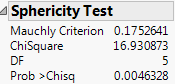
The sphericity test checks the appropriateness of an unadjusted univariate F test for the within-subject effects using the Mauchly criterion to test the sphericity assumption (Anderson 1958). The sphericity test and the univariate tests are always done using an orthonormalized M matrix. You interpret the sphericity test as follows:
• If the true covariance structure is spherical, you can use the unadjusted univariate F-tests.
• If the sphericity test is significant, the test suggests that the true covariance structure is not spherical. Therefore, you can use the multivariate or the adjusted univariate tests.
The univariate F statistic has an approximate F-distribution even without sphericity, but the degrees of freedom for numerator and denominator are reduced by some fraction epsilon (ε). Box (1954), Greenhouse and Geisser (1959), and Huynh-Feldt (1976) offer techniques for estimating the epsilon degrees-of-freedom adjustment. Muller and Barton (1989) recommend the Greenhouse-Geisser version, based on a study of power.
The epsilon adjusted tests in the multivariate report are labeled G-G (Greenhouse-Geisser) or H-F (Huynh-Feldt), with the epsilon adjustment shown in the value column.
Multivariate Model with Repeated Measures
One common use of multivariate fitting is to analyze data with repeated measures, also called longitudinal data. A subject is measured repeatedly across time, and the data are arranged so that each of the time measurements form a variable. Because of correlation between the measurements, data should not be stacked into a single column and analyzed as a univariate model unless the correlations form a pattern termed sphericity. See the previous section, “Univariate Tests and the Test for Sphericity”, for more details about this topic.
With repeated measures, the analysis is divided into two layers:
• Between-subject (or across-subject) effects are modeled by fitting the sum of the repeated measures columns to the model effects. This corresponds to using the Sum response function, which is an M-matrix that is a single vector of 1s.
• Within-subjects effects (repeated effects, or time effects) are modeled with a response function that fits differences in the repeated measures columns. This analysis can be done using the Contrast response function or any of the other similar differencing functions: Polynomial, Helmert, Profile, or Mean. When you model differences across the repeated measures, think of the differences as being a new within-subjects effect, usually time. When you fit effects in the model, interpret them as the interaction with the within-subjects effect. For example, the effect for Intercept becomes the Time (within-subject) effect, showing overall differences across the repeated measures. If you have an effect A, the within-subjects tests are interpreted to be the tests for the A*Time interaction, which model how the differences across repeated measures vary across the A effect.
Table 9.1 shows the relationship between the response function and the model effects compared with what a univariate model specification would be. Using both the Sum (between-subjects) and Contrast (within-subjects) models, you should be able to reconstruct the tests that would have resulted from stacking the responses into a single column and obtaining a standard univariate fit.
There is a direct and an indirect way to perform the repeated measures analyses:
• The direct way is to use the popup menu item Repeated Measures. This prompts you to name the effect that represents the within-subject effect across the repeated measures. Then it fits both the Contrast and the Sum response functions. An advantage of this way is that the effects are labeled appropriately with the within-subjects effect name.
• The indirect way is to specify the two response functions individually. First, do the Sum response function and second, do either Contrast or one of the other functions that model differences. You need to remember to associate the within-subjects effect with the model effects in the contrast fit.
Repeated Measures Example
For example, consider a study by Cole and Grizzle (1966). The results are in the Dogs.jmp table in the sample data folder. Sixteen dogs are assigned to four groups defined by variables drug and dep1, each having two levels. The dependent variable is the blood concentration of histamine at 0, 1, 3, and 5 minutes after injection of the drug. The log of the concentration is used to minimize the correlation between the mean and variance of the data.
1. Select Help > Sample Data Library and open Dogs.jmp.
2. Select Analyze > Fit Model.
3. Select LogHist0, LogHist1, LogHist3, and LogHist5 and click Y.
4. Select drug and dep1 and select Full Factorial from the Macros menu.
5. For Personality, select Manova.
6. Click Run.
7. In the Choose Response menu, select Repeated Measures.
Time should be entered for YName. If you check the Univariate Tests Also check box, the report includes univariate tests, which are calculated as if the responses were stacked into a single column.
8. Click OK.
Figure 9.9 Repeated Measures Window

Table 9.1 shows how the multivariate tests for a Sum and Contrast response designs correspond to how univariate tests would be labeled if the data for columns LogHist0, LogHist1, LogHist3, and LogHist5 were stacked into a single Y column, with the new rows identified with a nominal grouping variable, Time.
|
Sum M-Matrix
Between Subjects
|
Contrast M-Matrix
Within Subjects
|
||
|
Multivariate Test
|
Univariate Test
|
Multivariate Test
|
Univariate Test
|
|
intercept
|
intercept
|
intercept
|
time
|
|
drug
|
drug
|
drug
|
time*drug
|
|
depl
|
depl
|
depl
|
time*depl
|
The between-subjects analysis is produced first. This analysis is the same (except titling) as it would have been if Sum had been selected on the popup menu.
The within-subjects analysis is produced next. This analysis is the same (except titling) as it would have been if Contrast had been selected on the popup menu, though the within-subject effect name (Time) has been added to the effect names in the report. Note that the position formerly occupied by Intercept is Time, because the intercept term is estimating overall differences across the repeated measurements.
Example of a Compound Multivariate Model
JMP can handle data with layers of repeated measures. For example, see the Cholesterol.jmp data table. Groups of five subjects belong to one of four treatment groups called A, B, Control, and Placebo. Cholesterol was measured in the morning and again in the afternoon once a month for three months (the data are fictional). In this example, the response columns are arranged chronologically with time of day within month.
1. Select Help > Sample Data Library and open Cholesterol.jmp.
2. Select Analyze > Fit Model.
3. Select April AM, April PM, May AM, May PM, June AM, and June PM and click Y.
4. Select treatment and click Add.
5. Next to Personality, select Manova.
6. Click Run.
Figure 9.10 Treatment Graph

In the treatment graph, you can see that the four treatment groups began the study with very similar mean cholesterol values. The A and B treatment groups appear to have lower cholesterol values at the end of the trial period. The control and placebo groups remain unchanged.
7. Click on the Choose Response menu and select Compound.
Complete this window to tell JMP how the responses are arranged in the data table and the number of levels of each response. In the cholesterol example, the time of day columns are arranged within month. Therefore, you name time of day as one factor and the month effect as the other factor. Testing the interaction effect is optional.
8. Use the options in Figure 9.11 to complete the window.
Figure 9.11 Compound Window

9. Click OK.
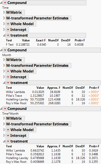
The tests for each effect appear. Parts of the report are shown in Figure 9.12. Note the following:
‒ The report for Time shows a p-value of 0.6038 for the interaction between Time and treatment, indicating that the interaction is not significant. This means that there is no evidence of a difference in treatment between AM and PM. Since Time has two levels (AM and PM) the exact F-test appears.
‒ The report for Month shows p-values of <.0001 for the interaction between Month and treatment, indicating that the interaction is significant. This suggests that the differences between treatment groups change depending on the month. The treatment graph in Figure 9.10 indicates no difference among the groups in April, but the difference between treatment types (A, B, Control, and Placebo) becomes large in May and even larger in June.
‒ The report for Time*Month shows no significant p-values for treatment. This indicates that the three-way interaction effect involving Time, Month, and treatment is not statistically significant.
Figure 9.12 Cholesterol Study Results
Discriminant Analysis
Discriminant analysis is a method of predicting some level of a one-way classification based on known values of the responses. The technique is based on how close a set of measurement variables are to the multivariate means of the levels being predicted. Discriminant analysis is more fully implemented using the Discriminant Platform (see the Discriminant Analysis chapter in the Multivariate Methods book).
In JMP you specify the measurement variables as Y effects and the classification variable as a single X effect. The multivariate fitting platform gives estimates of the means and the covariance matrix for the data, assuming that the covariances are the same for each group. You obtain discriminant information with the Save Discrim option in the popup menu next to the MANOVA platform name. This command saves distances and probabilities as columns in the current data table using the initial E and H matrices.
For a classification variable with k levels, JMP adds k distance columns, k classification probability columns, the predicted classification column, and two columns of other computational information to the current data table.
Example of the Save Discrim Option
Examine Fisher’s Iris data as found in Mardia, Kent, and Bibby (1979). There are k = 3 levels of species and four measures on each sample.
1. Select Help > Sample Data Library and open Iris.jmp.
2. Select Analyze > Fit Model.
3. Select Sepal length, Sepal width, Petal length, and Petal width and click Y.
4. Select Species and click Add.
5. Next to Personality, select Manova.
6. Click Run.
7. From the red triangle menu next to Manova Fit, select Save Discrim.
The following columns are added to the Iris.jmp sample data table:
SqDist[0]
Quadratic form needed in the Mahalanobis distance calculations.
SqDist[setosa]
Mahalanobis distance of the observation from the Setosa centroid.
SqDist[versicolor]
Mahalanobis distance of the observation from the Versicolor centroid.
SqDist[virginica]
Mahalanobis distance of the observation from the Virginica centroid.
Prob[0]
Sum of the negative exponentials of the Mahalanobis distances, used below.
Prob[setosa]
Probability of being in the Setosa category.
Prob[versicolor]
Probability of being in the Versicolor category.
Prob[virginica]
Probability of being in the Virginica category.
Pred Species
Species that is most likely from the probabilities.
Now you can use the new columns in the data table with other JMP platforms to summarize the discriminant analysis with reports and graphs. For example:
1. From the updated Iris.jmp data table (that contains the new columns) select Analyze > Fit Y by X.
2. Select Species and click Y, Response.
3. Select Pred Species and click X, Factor.
4. Click OK.
The Contingency Table summarizes the discriminant classifications. Three misclassifications are identified.
Figure 9.13 Contingency Table of Predicted and Actual Species

Statistical Details
This section gives formulas for the multivariate test statistics, describes the approximate F-tests, and provides details on canonical scores.
Multivariate Tests
In the following, E is the residual cross product matrix and H is the model cross product matrix. Diagonal elements of E are the residual sums of squares for each variable. Diagonal elements of H are the sums of squares for the model for each variable. In the discriminant analysis literature, E is often called W, where W stands for within.
Test statistics in the multivariate results tables are functions of the eigenvalues λ of  . The following list describes the computation of each test statistic.
Note: After specification of a response design, the initial E and H matrices are premultiplied by  and postmultiplied by M.
• Wilks’ Lambda

• Pillai’s Trace

• Hotelling-Lawley Trace

• Roy’s Max Root
E and H are defined as follows:
where b is the estimated vector for the model coefficients and A- denotes the generalized inverse of a matrix A.
The whole model L is a column of zeros (for the intercept) concatenated with an identity matrix having the number of rows and columns equal to the number of parameters in the model. L matrices for effects are subsets of rows from the whole model L matrix.
Approximate F-Tests
To compute F-values and degrees of freedom, let p be the rank of  . Let q be the rank of
  , where the L matrix identifies elements of
  associated with the effect being tested. Let v be the error degrees of freedom and s be the minimum of p and q. Also let
  and
and  .
.
Table 9.2, gives the computation of each approximate F from the corresponding test statistic.
|
Test
|
Approximate F
|
Numerator DF
|
Denominator DF
|
|
Wilks’ Lambda
|
 |
|
|
|
Pillai’s Trace
|
 |
|
|
|
Hotelling-Lawley Trace
|
 |
|
|
|
Roy’s Max Root
|
|
|
|
Canonical Details
The canonical correlations are computed as

The canonical Y’s are calculated as
where Y is the matrix of response variables, M is the response design matrix, and V is the matrix of eigenvectors of  for the given test. Canonical Y’s are saved for eigenvectors corresponding to eigenvalues larger than zero.
Details for Centroid Plot
The total sample centroid is computed as
Grand = 
where V is the matrix of eigenvectors of  .
.
The centroid values for effects are calculated as
and the vs are columns of V, the eigenvector matrix of  ,
,  refers to the multivariate least squares mean for the jth effect, g is the number of eigenvalues of
  greater than 0, and r is the rank of the X matrix.
The centroid radii for effects are calculated as
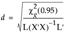
where g is the number of eigenvalues of  greater than 0 and the denominator L’s are from the multivariate least squares means calculations.
..................Content has been hidden....................
You can't read the all page of ebook, please click here login for view all page.