
Overview of Neural Networks
Think of a neural network as a function of a set of derived inputs, called hidden nodes. The hidden nodes are nonlinear functions of the original inputs. You can specify up to two layers of hidden nodes, with each layer containing as many hidden nodes as you want.
Figure 4.2 shows a two-layer neural network with three X variables and one Y variable. In this example, the first layer has two nodes, and each node is a function of all three nodes in the second layer. The second layer has three nodes, and all nodes are a function of the three X variables. The predicted Y variable is a function of both nodes in the first layer.
Figure 4.2 Neural Network Diagram
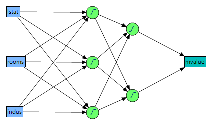
The functions applied at the nodes of the hidden layers are called activation functions. The activation function is a transformation of a linear combination of the X variables. For more details about the activation functions, see “Hidden Layer Structure”.
The function applied at the response is a linear combination (for continuous responses), or a logistic transformation (for nominal or ordinal responses).
The main advantage of a neural network model is that it can efficiently model different response surfaces. Given enough hidden nodes and layers, any surface can be approximated to any accuracy. The main disadvantage of a neural network model is that the results are not easily interpretable, since there are intermediate layers rather than a direct path from the X variables to the Y variables, as in the case of regular regression.
Launch the Neural Platform
To launch the Neural platform, select Analyze > Predictive Modeling > Neural.
Launching the Neural platform is a two-step process. First, enter your variables on the Neural launch window. Second, specify your options in the Model Launch control panel.
Use the Neural launch window to specify X and Y variables, a validation column, and to enable Informative Missing value coding.
Figure 4.3 The Neural Launch Window
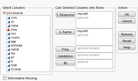
Y, Response
Choose the response variable. When multiple responses are specified, the models for the responses share all parameters in the hidden layers (those parameters not connected to the responses).
X, Factor
Choose the input variables.
Freq
Choose a frequency variable.
Choose a validation column. For more information, see “Validation Method”. If you click the Validation button with no columns selected in the Select Columns list, you can add a validation column to your data table. For more information about the Make Validation Column utility, see the Modeling Utilities chapter in the Predictive and Specialized Modeling book.
By
Choose a variable to create separate models for each level of the variable.
Check this box to enable informative coding of missing values. This coding allows estimation of a predictive model despite the presence of missing values. It is useful in situations where missing data are informative. If this option is not checked, rows with missing values are ignored.
For a continuous variable, missing values are replaced by the mean of the variable. Also, a missing value indicator, named <colname> Is Missing, is created and included in the model. If a variable is transformed using the Transform Covariates fitting option on the Model Launch control panel, missing values are replaced by the mean of the transformed variable.
For a categorical variable, missing values are treated as a separate level of that variable.
The Model Launch Control Panel
Use the Model Launch control panel to specify the validation method, the structure of the hidden layer, whether to use gradient boosting, and other fitting options.
Figure 4.4 The Model Launch Control Panel
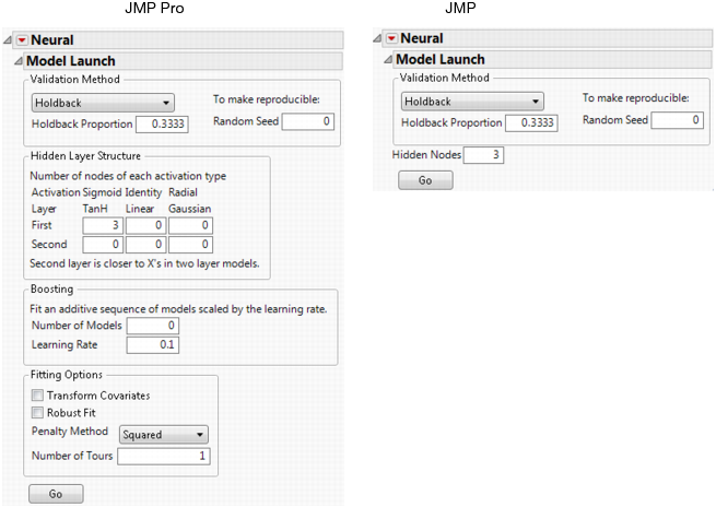
Validation Method
Select the method that you want to use for model validation. For details, see “Validation Method”.
Random Seed
Specify a nonzero numeric random seed if you want to reproduce the validation assignment for future launches of the Neural platform. By default, the Random Seed is set to zero, which does not produce reproducible results. When you save the analysis to a script, the random seed that you enter is saved to the script.
Hidden Layer Structure or Hidden Nodes
Specify the number of hidden nodes of each type in each layer. For details, see “Hidden Layer Structure”.
Note: The standard edition of JMP uses only the TanH activation function, and can fit only neural networks with one hidden layer.
Specify options for gradient boosting. For details, see “Boosting”.
Specify options for variable transformation and model fitting. For details, see “Fitting Options”.
Go
Fits the neural network model and shows the model reports.
After you click Go to fit a model, you can reopen the Model Launch Control Panel and change the settings to fit another model.
Validation Method
Neural networks are very flexible models and have a tendency to overfit data. When that happens, the model predicts the fitted data very well, but predicts future observations poorly. To mitigate overfitting, the Neural platform does the following:
• applies a penalty on the model parameters
• uses an independent data set to assess the predictive power of the model
Validation is the process of using part of a data set to estimate model parameters, and using the other part to assess the predictive ability of the model.
• The training set is the part that estimates model parameters.
• The validation set is the part that estimates the optimal value of the penalty, and assesses or validates the predictive ability of the model.
• The test set is a final, independent assessment of the model’s predictive ability. The test set is available only when using a validation column.
The training, validation, and test sets are created by subsetting the original data into parts. Select one of the following methods to subset a data set.
Excluded Rows Holdback
Uses row states to subset the data. Rows that are unexcluded are used as the training set, and excluded rows are used as the validation set.
For more information about using row states and how to exclude rows, see the Enter and Edit Data chapter in the Using JMP book.
Holdback
Randomly divides the original data into the training and validation sets. You can specify the proportion of the original data to use as the validation set (holdback).
KFold
Divides the original data into K subsets. In turn, each of the K sets is used to validate the model fit on the rest of the data, fitting a total of K models. The model giving the best validation statistic is chosen as the final model.
This method is best for small data sets, because it makes efficient use of limited amounts of data.
Uses the column’s values to divide the data into parts. The column is assigned using the Validation role on the Neural launch window. See Figure 4.3.
The column’s values determine how the data is split, and what method is used for validation:
‒ If the column has three unique values, then:
the smallest value is used for the Training set.
the middle value is used for the Validation set.
the largest value is used for the Test set.
‒ If the column has two unique values, then only Training and Validation sets are used.
‒ If the column has more than three unique values, then K-Fold validation is performed.
Hidden Layer Structure
Note: The standard edition of JMP uses only the TanH activation function, and can fit only neural networks with one hidden layer.
The Neural platform can fit one or two-layer neural networks. Increasing the number of nodes in the first layer, or adding a second layer, makes the neural network more flexible. You can add an unlimited number of nodes to either layer. The second layer nodes are functions of the X variables. The first layer nodes are functions of the second layer nodes. The Y variables are functions of the first layer nodes.
The functions applied at the nodes of the hidden layers are called activation functions. An activation function is a transformation of a linear combination of the X variables. The following activation functions are available:
TanH
The hyperbolic tangent function is a sigmoid function. TanH transforms values to be between -1 and 1, and is the centered and scaled version of the logistic function. The hyperbolic tangent function is:

where x is a linear combination of the X variables.
Linear
The identity function. The linear combination of the X variables is not transformed.
The Linear activation function is most often used in conjunction with one of the non-linear activation functions. In this case, the Linear activation function is placed in the second layer, and the non-linear activation functions are placed in the first layer. This is useful if you want to first reduce the dimensionality of the X variables, and then have a nonlinear model for the Y variables.
For a continuous Y variable, if only Linear activation functions are used, the model for the Y variable reduces to a linear combination of the X variables. For a nominal or ordinal Y variable, the model reduces to a logistic regression.
Gaussian
The Gaussian function. Use this option for radial basis function behavior, or when the response surface is Gaussian (normal) in shape. The Gaussian function is:
where x is a linear combination of the X variables.
Boosting
Boosting is often faster than fitting a single large model. However, the base model should be a 1 to 2 node single-layer model, or else the benefit of faster fitting can be lost if a large number of models is specified.
Use the Boosting panel in the Model Launch control panel to specify the number of component models and the learning rate. Use the Hidden Layer Structure panel in the Model Launch control panel to specify the structure of the base model.
The learning rate must be 0 < r ≤ 1. Learning rates close to 1 result in faster convergence on a final model, but also have a higher tendency to overfit data. Use learning rates close to 1 when a small Number of Models is specified.
As an example of how boosting works, suppose you specify a base model consisting of one layer and two nodes, with the number of models equal to eight. The first step is to fit a one-layer, two-node model. The predicted values from that model are scaled by the learning rate, then subtracted from the actual values to form a scaled residual. The next step is to fit a different one-layer, two-node model on the scaled residuals of the previous model. This process continues until eight models are fit, or until the addition of another model fails to improve the validation statistic. The component models are combined to form the final, large model. In this example, if six models are fit before stopping, the final model consists of one layer and 2 x 6 = 12 nodes.
Fitting Options
Transform Covariates
Transforms all continuous variables to near normality using either the Johnson Su or Johnson Sb distribution. Transforming the continuous variables helps mitigate the negative effects of outliers or heavily skewed distributions.
See the Save Transformed Covariates option in “Model Options”.
Robust Fit
Trains the model using least absolute deviations instead of least squares. This option is useful if you want to minimize the impact of response outliers. This option is available only for continuous responses.
Penalty Method
Choose the penalty method. To mitigate the tendency neural networks have to overfit data, the fitting process incorporates a penalty on the likelihood. See “Penalty Method”.
Number of Tours
Specify the number of times to restart the fitting process, with each iteration using different random starting points for the parameter estimates. The iteration with the best validation statistic is chosen as the final model.
Penalty Method
The penalty is  , where λ is the penalty parameter, and p( ) is a function of the parameter estimates, called the penalty function. Validation is used to find the optimal value of the penalty parameter.
|
Method
|
Penalty Function
|
Description
|
|
Squared
|
|
Use this method if you think that most of your X variables are contributing to the predictive ability of the model.
|
|
Absolute
|
|
Use either of these methods if you have a large number of X variables, and you think that a few of them contribute more than others to the predictive ability of the model.
|
|
Weight Decay
|
 |
|
|
NoPenalty
|
none
|
Does not use a penalty. You can use this option if you have a large amount of data and you want the fitting process to go quickly. However, this option can lead to models with lower predictive performance than models that use a penalty.
|
Model Reports
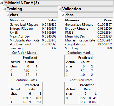
A model report is created for every neural network model. Measures of fit appear for the training and validation sets. Additionally, confusion statistics appear when the response is nominal or ordinal.
Figure 4.5 Example of a Neural Model Report
Training and Validation Measures of Fit
Measures of fit appear for the training and validation sets. See Figure 4.5.
Generalized RSquare
A measure that can be applied to general regression models. It is based on the likelihood function L and is scaled to have a maximum value of 1. The value is 1 for a perfect model, and 0 for a model no better than a constant model. The Generalized RSquare measure simplifies to the traditional RSquare for continuous normal responses in the standard least squares setting. Generalized RSquare is also known as the Nagelkerke or Craig and Uhler R2, which is a normalized version of Cox and Snell’s pseudo R2. See Nagelkerke (1991).
Entropy RSquare
Compares the log-likelihoods from the fitted model and the constant probability model. Appears only when the response is nominal or ordinal.
RSquare
Gives the RSquare for the model.
RMSE
Gives the root mean square error. When the response is nominal or ordinal, the differences are between 1 and p (the fitted probability for the response level that actually occurred).
Mean Abs Dev
The average of the absolute values of the differences between the response and the predicted response. When the response is nominal or ordinal, the differences are between 1 and p (the fitted probability for the response level that actually occurred).
Misclassification Rate
The rate for which the response category with the highest fitted probability is not the observed category. Appears only when the response is nominal or ordinal.
-LogLikelihood
Gives the negative of the log-likelihood. See the Fitting Linear Models book.
SSE
Gives the error sums of squares. Available only when the response is continuous.
Sum Freq
Gives the number of observations that are used. If you specified a Freq variable in the Neural launch window, Sum Freq gives the sum of the frequency column.
If there are multiple responses, fit statistics are given for each response, and an overall Generalized RSquare and negative Log-Likelihood is given.
Confusion Statistics
For nominal or ordinal responses, a Confusion Matrix report and Confusion Rates report is given. See Figure 4.5. The Confusion Matrix report shows a two-way classification of the actual response levels and the predicted response levels. For a categorical response, the predicted level is the one with the highest predicted probability. The Confusion Rates report is equal to the Confusion Matrix report, with the numbers divided by the row totals.
Model Options
Each model report has a red triangle menu containing options for producing additional output or saving results. The model report red triangle menu provides the following options:
Diagram
Shows a diagram representing the hidden layer structure.
Show Estimates
Shows the parameter estimates in a report.
Profiler
Launches the Prediction Profiler. For nominal or ordinal responses, each response level is represented by a separate row in the Prediction Profiler. For details about the options in the red triangle menu, see the Profiler chapter in the Profilers book.
Categorical Profiler
Launches the Prediction Profiler. Similar to the Profiler option, except that all categorical probabilities are combined into a single profiler row. Available only for nominal or ordinal responses. For details about the options in the red triangle menu, see the Profiler chapter in the Profilers book
Contour Profiler
Launches the Contour Profiler. This is available only when the model contains more than one continuous factor. For details about the options in the red triangle menu, see the Contour Profiler chapter in the Profilers book
Surface Profiler
Launches the Surface Profiler. This is available only when the model contains more than one continuous factor. For details about the options in the red triangle menu, see the Surface Plot chapter in the Profilers book.
ROC Curve
Creates an ROC curve. Available only for nominal or ordinal responses. For details about ROC Curves, see “ROC Curve” in the “Partition Models” chapter.
Lift Curve
Creates a lift curve. Available only for nominal or ordinal responses. For details about Lift Curves, see “Lift Curve” in the “Partition Models” chapter.
Plot Actual by Predicted
Plots the actual versus the predicted response. Available only for continuous responses.
Plot Residual by Predicted
Plots the residuals versus the predicted responses. Available only for continuous responses.
Save Formulas
Creates new columns in the data table containing formulas for the predicted response and the hidden layer nodes.
Save Profile Formulas
Creates new columns in the data table containing formulas for the predicted response. Formulas for the hidden layer nodes are embedded in this formula. This option produces formulas that can be used by the Flash version of the Profiler.
Save Fast Formulas
Creates new columns in the data table containing formulas for the predicted response. Formulas for the hidden layer nodes are embedded in this formula. This option produces formulas that evaluate faster than the other options, but cannot be used in the Flash version of the Profiler.
Creates prediction formulas and saves them as formula column scripts in the Formula Depot platform. If a Formula Depot report is not open, this option creates a Formula Depot report. See the “Formula Depot” chapter.
Make SAS Data Step
Creates SAS code that you can use to score a new data set.
Save Validation
Creates a new column in the data table that identifies which rows were used in the training and validation sets. This option is not available when a Validation column is specified on the Neural launch window. See “The Neural Launch Window”.
Creates new columns in the data table showing the transformed covariates. The columns contain formulas that show the transformations. This option is available only when the Transform Covariates option is checked on the Model Launch control panel. See “Fitting Options”.
Remove Fit
Removes the entire model report.
Example of a Neural Network
This example uses the Boston Housing.jmp data table. Suppose you want to create a model to predict the median home value as a function of several demographic characteristics. Follow the steps below to build the neural network model:
1. Launch the Neural platform by selecting Analyze > Predictive Modeling > Neural.
2. Assign mvalue to the Y, Response role.
3. Assign the other columns (crim through lstat) to the X, Factor role.
4. Click OK.
5. Enter 0.2 for the Holdback Proportion.
6. Enter 1234 for the Random Seed.
Note: In general, results vary due to the random nature of choosing a validation set. Entering the seed above enable you to reproduce the results shown in this example.
7. Enter 3 for the number of TanH nodes in the first layer.
8. Check the Transform Covariates option.
9. Click Go.
The report is shown in Figure 4.6.
Figure 4.6 Neural Report
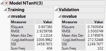
Results are provided for both the training and validation sets. Use the results of the validation set as a representation of the model’s predictive power on future observations.
The R-Square statistic for the Validation set is 0.819, signifying that the model is predicting well on data not used to train the model. As an additional assessment of model fit, select Plot Actual by Predicted from the Model red-triangle menu. The plot is shown in Figure 4.7.
Figure 4.7 Actual by Predicted Plot
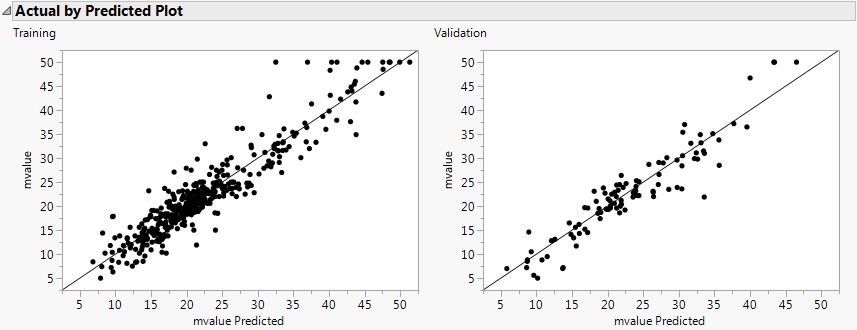
The points fall along the line, signifying that the predicted values are similar to the actual values.
To get a general understanding of how the X variables are impacting the predicted values, select Profiler from the Model red-triangle menu. The profiler is shown in Figure 4.8.
Figure 4.8 Profiler
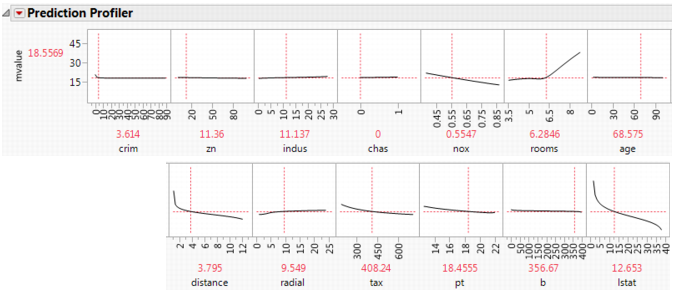
Some of the variables have profiles with positive slopes, and some negative. For example, rooms has a positive slope. This indicates that the more rooms a home has, the higher the predicted median value. The variable pt is the pupil teacher ratio by town. This variable has a negative slope, indicating that the higher the pupil to teacher ratio, the lower the median value.
..................Content has been hidden....................
You can't read the all page of ebook, please click here login for view all page.