
Chapter 3
Models with Factorial Treatment Designs
Our focus in this chapter bends slightly away from mixed models directly to investigate what is arguably the most common treatment design used in conjunction with mixed models —the factorial treatment design. We will start with an introduction to factorial designs in a simple randomized complete block experiment. Then we will bring ourselves back to mixed model territory with the split-plot design. The factorial treatment design in conjunction with variations of the basic split-plot experiment design is probably the most common form of mixed model.
3.1 Motivating Examples
Tensile Strength — A fabric manufacturer wants to test the tensile strength of a fabric after washing under various conditions. She has three machines available each with a setting for temperature, hot and cold, and for water level, high and low. It is possible that both temperature and water level affect the strength of the fabric.
Greenhouse — A plant researcher has two plant varieties and a pesticide meant to protect the plants against disease. In the greenhouse, the pesticide can only be applied to large sections of the benches. The bench sections can hold multiple plants. The researcher wants to identify the best plant and pesticide combination for disease resistance.
Semiconductor — A semiconductor engineer has several process conditions that affect resistance on the wafers produced. The position of the chips on the wafer can also affect resistance. The engineer wants to minimize resistance and understand the effects of process condition and position.
3.2 Conceptual Background
The examples discussed in Chapter 2 all had a single treatment factor of interest. Many times researchers have more than one treatment factor that they can control that could affect the response. Those researchers could run multiple experiments, one for each factor, but this is inefficient in both resources (time, equipment, etc.) and statistical efficiency. Specifically, when the experiments are run separately, the possibility of interaction between the treatment factors cannot be tested.
Key Terminology
Main Effect The effect of a single factor averaging over any other factors in the model.
Simple Effect The effect of one factor given a particular level of another factor.
Interaction An interaction occurs when the effect of one factor changes depending on the level of another factor. If the simple effect of a factor is different depending on which level of the other factor is used, then there is an interaction between the two factors.
The potential for interaction between two or more factors means we should design experiments to measure the interaction. The presence of an interaction typically restricts any further treatment comparisons tested after the initial interaction test. We will see how this works in the examples.
When there are two or more treatment factors, and one is harder to change than the other, a particular experiment design is natural. This design is the split-plot experiment design (and all of its more complicated relatives, the split-split plot, the split-strip plot, etc.).
In the split-plot design, the hard-to-change factor is assigned to the larger experimental unit, known as the whole plot. This assignment can be done either in a completely randomized manner (in a CRD) or when there is a need to block, in some form of a blocked design (RCBD, BIBD, etc.). Each of the whole plot units are then subdivided into split-plot units to which the easy-to-change factor is assigned.
The greenhouse example is a true split-plot. The sections of the greenhouse benches are whole plots to which the amount of pesticide is applied. Within those sections, the placement of the two plant varieties is randomized to the "split" section.
In the semiconductor example described above, process conditions can only be applied to whole wafers. Therefore wafer is the whole plot experimental unit. The individual chips are physical subdivisions of the whole wafer and thus split the whole plot. The position treatment is assigned to the split-plot chips. Technically speaking, position is not a true split-plot effect as position is the same on all wafers and not randomized. The analysis, however, is the same.
3.3 RCBD with Factorial Treatments, Tensile Strength Example
The following example explores the tensile strength of fabric under differing care conditions. These data are in a file called Tensile Strength.jmp. The manufacturer has three washing machines available for this test. Each machine has settings for Temperature, cold and hot, and Water level, low and high. Both temperature and water level could affect the measured strength of the fabric, and there may be variability as a result of the particular machine used.
Each washing machine can have only one setting for each of temperature and water level for a particular run. Each machine can be run four times in the time allotted for the experiment. This naturally creates blocks of size four to which the combinations of temperature and water level can be randomized to the runs. This is an RCBD with factorial treatments. Later in this chapter we will see a similar experiment design that requires a different analysis to correctly capture the way the treatments are randomized to the experimental units, so it is worth noting now how we can identify that we have an RCBD analysis and not a split-plot analysis in this example. In this case, we can see that it is the combination of the temperature and water level that are completely randomized to ANY of the four runs within a machine. There is no non-randomness to these treatment applications, except that all combinations must be present in all blocks. The blocks are the only feature restricting our randomization of the treatment application. In later examples in this chapter, we will see that the application of one treatment happens to groups of experimental units within blocks, and then the other treatment is applied randomly within those groups. This is the key difference to notice that will drive an analysis for RCBD with factorial treatments rather than the more complicated analysis of a split-plot. Let’s look at the ANOVA breakdown of our RCBD with factorial treatments.
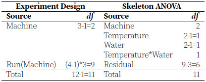
Machine is the block and within each block we perform four runs. The notation Run(Machine) is read "run within machine" and is an example of nesting of experimental units. Temperature and Water are the two main fixed effects, each with two levels, and we call this a 2×2 factorial. We write interaction effects using an asterisk (*), and Temperature*Water has a single degree of freedom obtained by multiplying the degrees of freedom of its constituent main effects. The statistical model based on the skeleton ANOVA above is as follows.
Model for the RCBD with Factorial Treatments, Tensile Strength
yijk =µ+ αi+βj +αβij +rk+eijk
yijk is the response of the ith temperature with the jth water level in the kth machine.
µ is the intercept.
αi is the effect of the ith level of Temperature.
βj is the effect of the jth level of Water level.
αβij is the effect of the ith Temperature with the jth Water level.
rk is the effect of the kth random block and
eijk is the residual error and eijk ~ N (0, σ2).
With our statistical model defined we can fit this model in JMP.
JMP Instructions for Tensile Strength
Go to Analyze > Fit Model.
Enter y as the Y variable. Note that the default personality becomes Standard Least Squares because you’ve entered a continuous variable in the Y role. Keep this default.
Enter Machine, Temperature and Water in the Construct Model Effects box.
Add the interaction of the Temperature and Water by selecting both from the list of Columns at the same time, and then click the Cross button to add this interaction to the Construct Model Effects box.
By default, these are all Fixed Effects. To make the Machine random, click on that variable in the Construct Model Effects box, select the Attributes drop-down, and select Random Effect. Click Run to fit the model.

Results and Interpretation
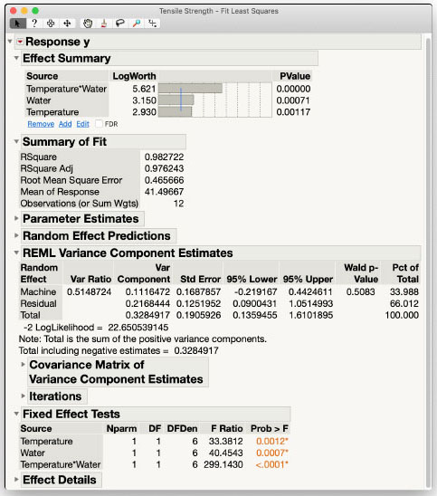
Looking first at the REML Variance Component Estimates in Figure 3.1 we see that the variance for Machine is approximately half the residual variance. The variance is also not significantly different from zero according to the Wald test. This is not concerning as we did not have very many machines available to estimate this variance, and the washing machine manufacturer would probably be glad to see that there is not much variability between machines.
The Fixed Effect Tests show that all of the fixed effects in the model, Temperature, Water and their interaction, are statistically significant. We can also verify that the degrees of freedom agree with our skeleton ANOVA table. Because the interaction effect is significant, the main effect tests for Water and Temperature should be interpreted very cautiously as they are effectively averaging over heterogeneous states. To break down the effects water and temperature have upon tensile strength, we look at simple effects. The next steps show what an interaction looks like graphically and how to investigate simple effects.
Figure 3.1: Initial Results for Tensile Strength
Interaction Plot of Temperature*Water Effect
To explore an interaction effect, expand the Effect Details report section, scroll down to the interaction effect, and select the LSMeans Plot for Temperature*Water from the red triangle menu. Check the box for Create an Interaction Plot and choose with Temperature as the overlay.

The Least Squares Means Plot in Figure 3.2 shows a classic interaction plot. When the water level is low, hot temperature results in higher tensile strength than cold. However, when the water level is high, the hot temperature results in a lower tensile strength than cold. These are the simple effects of temperature given a particular value of water level. Because the simple effects are different, there is an interaction.
Figure 3.2: Interaction Plot of Temperature*Water for Tensile Strength

Figure 3.3: Results of Slices of Temperature*Water in Tensile Strength

We see this with the crossing lines in the plot and is why the F test for Temperature*Water has a small p-value.
Based on the visual interaction plot and statistical results thus far, we would make the following preliminary conclusions for tensile strength. If water level is low, hot temperature will result in a higher tensile strength. If water level is high, then cold temperature will result in a higher tensile strength. To obtain formal statistical tests and estimates of the simple effects, choose Test Slices from the red triangle menu next to Temperature*Water. Results of these slices are shown in Figure 3.3 with the Test Detail where Water=low is expanded.
The formal tests confirm what we see in the interaction plot that all of the conditional slices are statistically significant. Looking specifically at the slice where the water level is held at low, we see that the difference between the hot and cold temperature tensile strengths is 3.0967 units with a standard error for that comparison of 0.38. We know that the hot temperature tensile strength is higher than the cold because hot,low has a coefficient of 1 and cold,low has a coefficient of -1. Similar information is available for the other slices.
The three unit difference was statistically significant. The researcher would be able to say whether this magnitude of difference is practically significant. Presumably, this experiment was designed for power to detect at least a certain difference, and this difference is both statistically and practically significant. We will discuss power and how to determine sample size in Chapter 8.
Note that the slices are not adjusted for multiple comparisons. You should typically have in mind a limited number of interesting slices before conducting this test in order to limit the familywise error inflation. When you are interested in many or all of the pairwise comparisons, the Tukey’s HSD option will appropriately adjust for multiple comparisons. Remember, though, that these p-values (adjusted or unadjusted) should not be used as hard rules but rather as pieces of evidence for a difference that should always be reported along with the size of that observed difference and an acknowledgement of the size of a difference that would actually be practical and important. However, in the presence of interactions, some of the comparisons in the Tukey’s HSD report are not considered valid comparisons. As soon as there is an interaction, any comparisons are restricted to where one of the factors is held at a particular level. In this example, comparing the LSMeans for the cold, low combination to the hot, high combination is disallowed because both factors are changing.
JMP Pro Instructions for Tensile Strength
Go to Analyze > Fit Model. Enter y as the Y variable. Change the default personality from Standard Least Squares to Mixed Model.
Select Temperature and Water in the Select Columns box then choose Full Factorial from the Macros list to add both fixed effects and the interaction to the Construct Model Effects box.
Enter Machine in the Random Effects tab of the Construct Model Effects box. Click Run to fit the model.

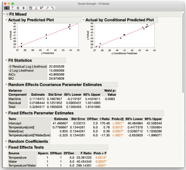
Figure 3.4: Fit Mixed Analysis of Tensile Strength
Results and Interpretation
The Fit Mixed results are the same as the Standard Least Squares personality analysis but include visuals of model fit in the Actual by Predicted and Actual by Conditional Predicted Plots. There are no obvious problems in the data based on these plots shown in Figure 3.4.
A key difference in using the Mixed Model personality comes when investigating the interaction effect further. We use the Multiple Comparisons option rather than having the Effect Details report section that the Standard Least Squares personality provides.
You can visualize the interaction plot in Fit Mixed using the Multiple Comparisons tool. Estimates > Multiple Comparisons under the red triangle menu brings up the Multiple Comparisons dialog box. Select Temperature*Water, check the Show Least Squares Means Plot box, check the Create an Interaction Plot box, and choose Temperature as the overlay term. The completed dialog box is shown in Figure 3.5.
Figure 3.5: Multiple Comparisons Dialog Box for Interaction Plot

After clicking OK, the interaction Least Squares Means Plot is added to the report. The plot is identical to before. The Multiple Comparisons tool in Fit Mixed does not have the same Slice capabilities that Standard Least Squares has, so within this personality we must carefully use the Tukey HSD pairwise comparisons available in the red triangle menu. This is shown in Figure 3.6.
Figure 3.6: Fit Mixed Analysis of Interaction in Tensile Strength
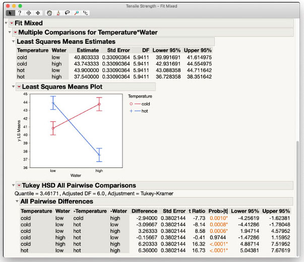
Again, due to the presence of the significant interaction, only four of the six comparisons presented are considered valid. One factor level must be held constant across the comparison. The differences, standard errors and p-values for the four valid comparisons match those obtained in the Slices option in Standard Least Squares.
3.4 Split-Plot Design, Greenhouse Example
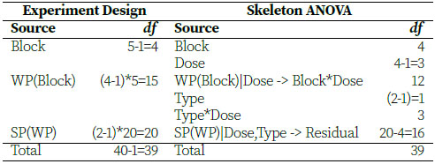
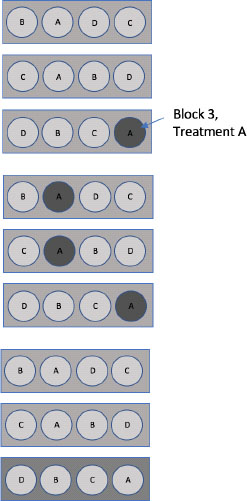
A plant researcher has two plant varieties and a pesticide meant to protect the plants against disease. In the greenhouse the amount of pesticide, Dose, can be applied to sections of the benches. Due to procedure and equipment, this is a hard-to-change factor, or whole plot factor, in this experiment. The bench sections can hold multiple plants, so the two varieties of plant, Type, are randomly assigned spaces within each bench section. This is an easy-to-change factor, the split-plot factor. Due to the natural variability within the greenhouse, whole benches serve as the blocking criterion, Block. Figure 3.7 shows an example randomization of the two treatment factors to one bench. The researcher wants to identify the best plant and pesticide combination for disease resistance. The data for this experiment are in the Variety-Pesticide Evaluation.jmp data table.
Figure 3.7: Example Bench with Pesticide Dose and Variety Type Randomized by a Split-Plot Design

Given the description of the experiment and the sketched example bench, we can create the skeleton ANOVA of this design, which will lead us to our model. For the experiment design, there are five benches serving as blocks, four whole plots within each block (twenty total whole plots), and two split-plots within each whole plot. Dose (of pesticide) is applied to the whole plots, and Type (variety of plant) and Type*Dose are observed at the split-plot level.
Using the terms in the Skeleton ANOVA, we can define the statistical model for this split-plot experiment and use JMP to analyze it.
Mixed Model for a Split-Plot Experiment
The statistical model for these data is
yijk=µ+rk+δi+wik+τj +δτij +eijk
yijk is the observation on the ith Dose, jth Type, and kth block.
µ is the intercept.
rk is the kth block effect, and
δi is the ith Dose effect.
wik is the ikth whole-plot (Block * Dose) effect, and
τj is the jth Type effect.
δτij is the ijth Dose*Type interaction effect.
eijk is the ijkth split-plot error and eijk ~ N (0, σ2).
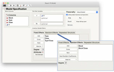
JMP Instructions for Greenhouse Example
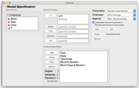
The Y column is the response variable Y. Add the model effects in the order of the statistical model shown above. Select the two columns Type and Dose, then use the Macros > Full Factorial macro. Next add the effect of Block. Select Block in the Construct Model Effects window then select Dose in the Columns list and click Cross to define the whole plot error term. (If we know the Block and the Dose level, we can uniquely identify which whole plot the observation is in.) Finally, select Block and Block*Dose and choose Attributes > Random Effect to designate them as random. The figure below shows the completed dialog box.
Results and Interpretation
Figure 3.8 shows the results of this analysis.
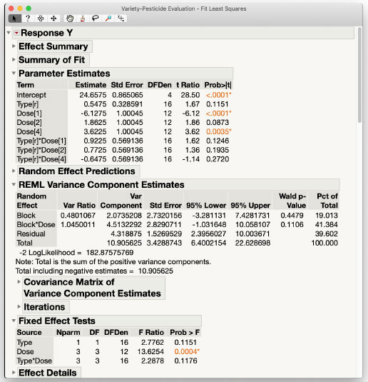
The Effect Summary section provides a quick visual indication of results for the fixed effects, indicating the primary action involves the main effect Dose. The Summary of Fit section provides basic model fitting statistics, and the Parameter Estimates section provides a breakdown of each individual fixed effects parameter.
The REML Variance Components section reveals that in partitioning of whole plot variance, bench-to-bench variability (Block) is approximately half of that within-bench (Block*Dose). Split-plot variability (Residual) is about the same as within-bench (Block*Dose). We therefore have approximately a 20:40:40 split attributable to these three sources of variability. The greenhouse manager may be interested in this breakdown and be able to offer further explanations in terms of the particular benches used and potential differences in delivery of resources like sunlight and irrigation.
Figure 3.8: Results for the Greenhouse Example
The interaction between plant Type and pesticide Dose appears to be negligible, though with multiple numerator degrees of freedom there may be an effect. Some researchers use a more lenient α-level, up to α = 0.20, in these situations to avoid the Type I error of concluding there is no interaction when, in fact, there is. We can investigate this further using the Multiple Comparisons tool under Estimates in the red triangle menu.
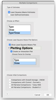
Multiple Comparisons of Type*Dose Effect
Choose Type*Dose in the Effects list of the Multiple Comparison window. Check the Show Least Squares Means Plot box. Then check the Create an Interaction Plot box and choose Dose for the overlay. The figure to the right shows the completed Multiple Comparisons window for the interaction plot.
The Least Squares Means Plot defaults to including confidence limits for the means. They can be turned off in the Least Squares Means Plot red triangle menu. Figure 3.9 shows the Multiple Comparisons report with the limits turned off. Visually, it appears that plant Type S has a lower response from plant Type R with Doses 1 and 2, but similar or higher responses with Doses 4 and 8. Combined with the p-value for the interaction test, it may be better to draw conclusions based on the interaction effects rather than the main effects.
To formally test differences of the interaction effects, we can choose All Pairwise Differences > Tukey HSD from the Multiple Comparisons red triangle menu. This adds every pairwise difference of the Type*Dose Least Squares Means. However, not all of these comparisons are valid in the presence of an interaction effect. Only comparisons where either the Type is held constant while Dose changes, or Dose is held constant while Type changes are valid. These are the simple effects. Based on the interaction plot, we focus first on the simple effects of Type given a Dose level.
For Dose 1, the difference between the resistant, r, and susceptible, s, varieties is 2.94, which is the largest difference between the Types at any Dose level. This is not a significant difference, however. You can conclude that regardless of Dose level, there is no difference in the response of the two Types.
Looking instead at the effect of Dose given a specified Type, we find some interesting effects. Given the resistant Type, Dose 1 results in a significantly lower response than Doses 2 and 4 (p-values 0.0128 and 0.0090, respectively) But there is no evidence of a statistical difference between Doses 1 and 8, 2 and 4, 2 and 8, or 4 and 8 (all p-values > 0.6298). Given the resistant Type, there are diminishing returns when increasing the pesticide Dose.
When holding Type constant at the susceptible variety, Dose 1 is significantly lower than all three other Dose levels (p-values 0.0094, 0.0004, and 0.0050, respectively). Like the resistant Type, the higher dose comparisons show no difference.
The alternate conclusion about the difference between Doses 1 and 8 with the two variety Types explains why the test for interaction was marginal. Whether that difference is important would be a decision for the plant researchers. However, given that Doses 2, 4, and 8 are not significantly different for either Type, it may be sufficient to conclude that a higher Dose of pesticide regardless of susceptibility of plant Type is required. That is what an analysis of the main effect of Dose would also conclude.
Figure 3.9: Multiple Comparisons for Type*Dose

JMP Pro Instructions for Greenhouse Example
The Y column is the response variable Y. Add the model effects in the order of the statistical model. For the Fixed Effects select the two columns Type and Dose, then use the Macros > Full Factorial macro. Switch to the Random Effects tab to add the remaining effects from the model. Add the effect of Block. Select Block in the Random Effects window then select Dose in the Columns list and click Cross to define the whole plot error term. If we know the Block and the Dose level, we can uniquely identify which whole plot the observation is in. The completed dialog box is shown below.
Results and Interpretation
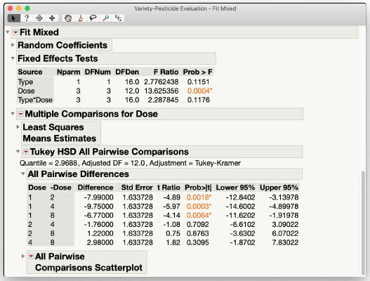
The results of the Mixed Model personality analysis are shown in Figure 3.10 and are the same as those shown in the previous section using the Standard Least Squares personality. The Type*Dose interaction is negligible, and the main effect of Type is also negligible at usual α-levels. We do have a significant main effect of Dose with p-value of 0.0004. We can investigate this effect further using Multiple Comparisons from the Fit Mixed red triangle menu. In the interest of space, the steps are not shown, but the results are included in Figure 3.11. Dose 1 results in a significantly lower response than the other three Doses (p-values 0.0018, 0.0003, and 0.0064, respectively). Those three Doses are not significantly different from each other, however, with all p-values > 0.3095. We can conclude that a Dose greater than Dose 1 is needed to improve the response of the plants, but more than Dose 2 may be unnecessary and potentially wasteful of the product and harmful to the environment.
Figure 3.10: Fit Mixed Report for the Variety-Pesticide Data
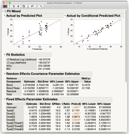
Figure 3.11: Fit Mixed Report for the Variety-Pesticide Data - Pairwise Differences
3.5 What About Interactions Between Fixed and Random Effects?
Generally, the interaction between a fixed effect and a random effect will not be of interest for statistical testing, but can be effective for modeling a source of variability. Be aware though, in cases such as the metal bonding example from Chapter 2, this interaction effect is completely confounded with residual errors, and should therefore not even be included in the model. On the other hand, if the treatment*block combinations are replicated, then it can be distinguished from residual variance and we can describe things about that interaction effect. But how? As a fixed effect? Or as a random effect?
Here we see an RCBD with no replication, where the interaction combinations are the smallest unit that receives the treatment application. We could name the block level and the treatment level to completely identify any experimental unit. Notice that this also means that we have the same number of interaction combinations as we have experimental units for the whole experiment.
Looking more closely at this design, we see that there are three replicates, each in different blocks, that will lend themselves to an estimate and a test of the Treatment A effect.
We see that there are four replicates, all in a single block but given the four different treatments, that allow us to make an estimate and get a statistical test of the Block 3 effect.
But when we have no replication for the interaction effect between the blocks and the treatment, we are not able to get a statistical test for that effect. We need at least two observations at the same factor combination in order to get an estimate of the corresponding variance. Without a variance estimate, we cannot do traditional statistical testing.
Here we see the same experimental and treatment design, but with replication at the block*treatment level.

Now we have twice as many experimental units as we have treatment*block combinations, and just specifying a certain treatment*block combination identifies two experimental units instead of a single experimental unit. We now have replication at the interaction level, so we can now estimate that interaction effect if we want to do so.
The next question, though, is “Do we want to estimate that interaction effect, even if we have the replication that allows it?”
Remember that a conceptual difference between random and fixed effects is that we consider the levels of the random effect to be (at least approximately) randomly sampled from a larger set of possible levels, so it is usually not interesting to test differences between these random levels. The same is true for the interactions between a random and a fixed effect. If you did not care about making comparisons between the blocks in an RCBD, then you likely also do not care about making comparisons between the block-by-treatment combinations. By treating the interaction of a fixed effect with a random effect as random, the focus of that effect is on the contribution to explaining variation, rather than on making means comparisons as we would for a fixed-by-fixed interaction.
It can be helpful to think about the randomness attribute of a factor as a contagious disease – if a factor is random, then any interactions that include that factor will also be random. A typical mixed model would be as follows:
Statistical Model: One Fixed, One Random, and Their (Random) Interaction
The statistical model with replication inside the block*treatment interaction and with the block*treatment interaction included in the model is
yijk =µ+αi+rj +αrij +eijk
yijk is the continuous response variable.
αi is the effect of the ith level of the treatment.
rj is the effect of the jth level of the random (blocking) factor and
αrij is the effect of the ith level of the treatment at the jth level of the random (blocking) factor and
eijk is the residual error and eijk ~ N (0, σ2).
This model requires replication within the interaction. That is, there must be multiple observations for any single combination of the ith level of the treatment at the rth level of the random (blocking) factor.
One final note about interactions between fixed and random effects: we often find that experimental units are different for different treatment factors within the same experiment. When deciding whether to include a mixed interaction term, think about the experimental unit for each treatment separately. You still might include a mixed interaction effect that is equivalent to the experimental unit for one treatment factor but has replication for another treatment factor. In fact, this is exactly what we do for split-plot-style experiments. To illustrate this further, let’s now consider another form of split-plot experiment that uses nesting.
3.6 Nested Design, Semiconductor Example
The Semiconductor Experiment.jmp data table contains the results of the semiconductor experiment described at the beginning of this chapter. The column Wafer contains identifiers for the twelve randomly selected wafers from a lot. Importantly, note how Wafer is coded in the table. Wafer only includes the numbers 1, 2, and 3, and those values repeat for each of the process conditions, ET. However, Wafer 1 with ET 1 is not the same as Wafer 1 with ET 2. Therefore, Wafer is nested within levels of ET and is the experimental unit for ET. Resistance is measured at four Position locations on each Wafer. The ANOVA is as follows:
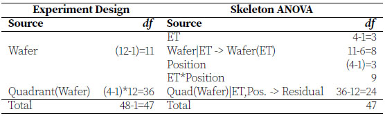
This is a two-way factorial treatment design with factors ET and Position, but the experimental units are different for each. We label this example "Nested Design" to emphasize how Wafer is coded, but it is also a split-plot design with ET as the whole-plot (hard-to-change) factor and Position as the subplot (easy-to-change) factor. Wafer denotes the whole-plot experimental units for ET, and Quadrant(Wafer) denotes the subplot experimental units for Position and ET*Position.
Mixed Model for the Nested Design, Semiconductor Example
The statistical model for these data is
yijk=µ+αi+wij +βk+(αβ)ik+ eijk
yijk is the Resistance measured at the kth Position on the jth Wafer in the ith level of ET.
αi is the effect of the ith level of ET.
wij is the effect of the jth Wafer in the ith ET, and
βk is the effect of the kth level of Position.
(αβ)ik is the interaction between the ith level of ET and kth Position.
eijk is the residual error and eijk ~ N (0, σ2).
JMP Instructions for Semiconductor Experiment.jmp example
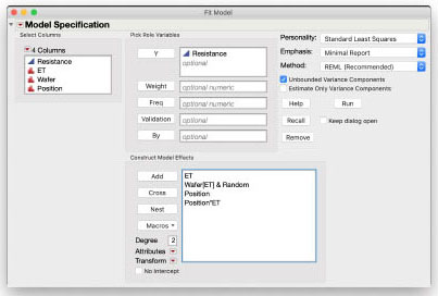
Below is the completed Fit Model dialog box. Resistance is the Y variable. ET, Wafer and Position. are the Model Effects. Because Wafer is nested within ET, select Wafer in the Model Effects and select ET in the Select Columns section, and then click the Nest button. Wafer in the Model Effects is now Wafer[ET]. This is the standard notation for a nested effect: we say “Wafer nested in ET” and we denote this with InsideEffect[OutsideEffect] (see Tip Box, below). This effect is also the whole plot error term and must be random. With it selected, choose Attributes > Random Effect to designate it as random. To add the interaction term for ET and Position, select Position in the Model Effects and select ET in Select Columns, then click the Cross button. The effect Position*ET is added to the Model Effects list. Click the Run button to fit the model.
Tip Box
The notation of nested effects is often a point of confusion for new Mixed Modelers. We always say “Effect A is nested in Effect B” and write A[B]. If we took a sample of randomly selected potato chip samples from different supplier plants, we would say that the potato chip samples are nested in the supplier plant, and we would write this PotatoChipSample[SupplierPlant]. We go first to the Supplier Plant, and then we sample within it to get the Potato Chips Samples, so some people feel that the order of the notation is “backwards.” It might help to think of the logic this way: you are writing down the effect, A, (or “PotatoChipSamples”), and you want to give yourself a parenthetical reminder that it is actually nested inside another Effect, B, (or “SupplierPlant”), hence A[B], or PotatoChipSample[SupplierPlant].
Results and Interpretation
The analysis of these data is shown in Figure 3.12.
In the REML Variance Component Estimates table you see that the variability among Wafers (the Wafer[ET] Variance Component) is approximately the same as residual variability within Wafer (the Residual Variance Component), each contributing half of the total variability in the data after accounting for fixed effects. The Fixed Effects Tests table shows that there is not a significant interaction between Position and ET (p=0.6125), nor is there a significant main effect of ET (p = 0.2015). You can see that the denominator degrees of freedom for the test of ET is 8, as it is properly using the Wafer[ET] whole plot variance for its error term. The lack of statistical significance is evidence for a small effect that likely is not strictly zero. If the engineers at the semiconductor plant believe ET truly affects Resistance, the variance estimates from this experiment can be used to conduct a power analysis to determine the number of wafers necessary to detect a significant difference with a predefined magnitude.
Figure 3.12: Standard Least Squares Report for the Semiconductor Experiment Data
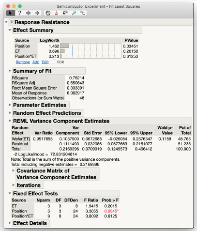
Similar considerations apply to the Position*ET interaction. One of the main questions the engineers have is whether there is any type of interaction between the two effects. We have the statistical answer to this question from this Fixed Effects Test output: the test for the Position*ET interaction is not statistically significant. However, we may still want to explore the magnitude of the effect, despite it not being statistically significant.
You can visualize the interaction plot from within the Multiple Comparisons tool. Estimates > Multiple Comparisons under the red triangle menu brings up the Multiple Comparisons dialog box. Select Position*ET, check the Show Least Squares Means Plot box, check the Create an Interaction Plot box, and choose Position as the overlay term. The completed dialog box is shown in Figure 3.13.
Figure 3.13: Multiple Comparisons Dialog Box for Interaction Plot

After clicking OK, the Multiple Comparisons for Position*ET section is added to the report. It includes a table of the Least Squares Means Estimates as well as the Least Squares Means Plot. The error bars on the plot can obscure the visualization of the interaction, so you can turn them off by selecting Show Confidence Limits from the Least Squares Means Plot red triangle menu. The plot without the confidence bars is shown in Figure 3.14.
Figure 3.14: Interaction Plot for the Semiconductor Experiment Data
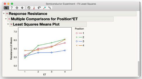
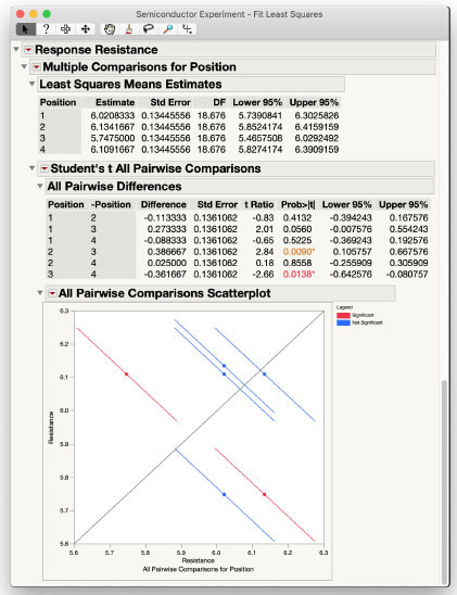
While the lines for Position cross a little from one level of ET to the next, it does appear that the effect of ET is the same regardless of Position; that is, the lines are approximately parallel to each other. This visually confirms the statistical test initially performed. The plot also shows that for all types of ET except 1, Position 3 has the lowest resistance measurement. You can confirm the difference is significant using Multiple Comparisons of just the Position effect. The dialog box for this comparison is shown in Figure 3.15.
Figure 3.15: Multiple Comparison Dialog for Least Squares Means of Position

The results of these comparisons are shown in Figure 3.16. You can see in the All Pairwise Differences table that Position 3 has significantly less resistance than both Position 2 and Position 4. Position 3 would have significantly less resistance than Position 1 with a slightly relaxed α-level of α =0.0560.
In previous examples, we used the Tukey correction to control the familywise error rate, but we did not in this example. To use or not use the correction method is a choice the analyst must make weighing the design of the study, the purpose of the study, and the number of comparisons being made. If the design was powered for the type and number of comparisons made (that is, these comparisons were pre-planned and not post-hoc), typically no correction would be used as that works against the design. If a study is a preliminary, exploratory experiment where the researchers are looking for any possible treatment to move on to further study, adjustments would not be used as they make things “less significant” and a potential treatment might be overlooked. If making a Type 1 error would have negative consequences, using the correction would be recommended. For this example, despite the comparisons being post-hoc, we chose not to use the correction as the number of comparisons was small and the risks of a Type 1 error were negligible.
Figure 3.16: Least Squares Means Differences of Position
JMP Pro Instructions for Semiconductor Experiment.jmp Example
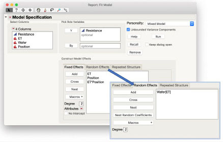
As this is a factorial experiment with the two factors ET and Position, you can use the Macros > Full Factorial macro when using the Mixed Model personality of Fit Model. That completes the Fixed Effects tab of the launch dialog box. The Random Effects tab gets the term identifying the whole plot variance, Wafer[ET]. Add Wafer to the Random Effects. Select it in the Random Effects window and select ET in the columns window, and then click the Nest button to nest the Wafers within ET. The completed dialog box is shown below.
Results and Interpretation
Figure 3.17 shows the results of the analysis from the completed dialog box.
The Actual by Predicted Plot and Actual by Conditional Predicted Report indicate a reasonable fit for this model to these data. The Random Effects Covariance Parameter Estimates table shows the estimates and standard errors of the two variance components, the whole plot Wafer[ET] and residual variance, approximately equal. The Fixed Effects Tests table shows the same results as in Standard Least Squares with no significant effects of the interaction between ET and Position and a mildly significant main effect of Position.
The remainder of the analysis to answer the engineer’s questions can be performed the same way as in the previous Standard Least Squares personality section.
Figure 3.17: Fit Mixed Report for the Semiconductor Experiment Data

3.7 Exercises
1. In the tensile strength example, what are the experimental units to which treatments are applied? How does this compare to treatment assignment in a split-plot design?
2. In the semiconductor example, recode the levels of Wafer in the table so that they are no longer nested within ET, and rerun the analysis. What changes in the results?