The first of these categories is the microbenchmark. A microbenchmark is a test designed to measure a very small unit of performance: the time to call a synchronized method vs. a non-synchronized method; the overhead in creating a thread vs. using a thread pool; the time to execute one arithmetic algorithm vs. an alternate implementation; and so on.

Microbenchmarks may seem like a good idea, but they are very difficult to write correctly. Consider the following code, which is an attempt to write a microbenchmark that tests the performance of different implementations of a method to compute the Nth Fibonacci number:

public void doTest() {
    // Main Loop
    double l;
    long then = System.currentTimeMillis();
    for (int i = 0; i < nLoops; i++) {
        l = fibImpl1(50);
    }
    long now = System.currentTimeMillis();
    System.out.println("Elapsed time: " + (now - then));
}
...
private double fibImpl1(int n) {
    if (n < 0) throw new IllegalArgumentException("Must be > 0");
    if (n == 0) return 0d;
    if (n == 1) return 1d;
    double d = fibImpl1(n - 2) + fibImpl(n  - 1);
    if (Double.isInfinite(d)) throw new ArithmeticException("Overflow");
    return d;
}

This may seem simple, but there are many problems with this code.

long then = System.currentTimeMillis();
long now = System.currentTimeMillis();
System.out.println("Elapsed time: " + (now - then));

for (int i = 0; i < nLoops; i++) {
    l = fibImpl1(random.nextInteger());
}

int[] input = new int[nLoops];
for (int i = 0; i < nLoops; i++) {
    input[i] = random.nextInt();
}
long then = System.currentTimeMillis();
for (int i = 0; i < nLoops; i++) {
    try {
        l = fibImpl1(input[i]);
    } catch (IllegalArgumentException iae) {
    }
}
long now = System.currentTimeMillis();

public double fibImplSlow(int n) {
    if (n < 0) throw new IllegalArgumentException("Must be > 0");
    if (n > 1476) throw new ArithmeticException("Must be < 1476");
    return verySlowImpl(n);
}

package net.sdo;

import java.util.Random;

public class FibonacciTest {
    private volatile double l;
    private int nLoops;
    private int[] input;

    public static void main(String[] args) {
        FibonacciTest ft = new FibonacciTest(Integer.parseInt(args[0]));
        ft.doTest(true);
        ft.doTest(false);
    }

    private FibonacciTest(int n) {
        nLoops = n;
        input = new int[nLoops];
        Random r = new Random();
        for (int i = 0; i < nLoops; i++) {
            input[i] = r.nextInt(100);
        }
    }

    private void doTest(boolean isWarmup) {
        long then = System.currentTimeMillis();
        for (int i = 0; i < nLoops; i++) {
            l = fibImpl1(input[i]);
        }
        if (!isWarmup) {
            long now = System.currentTimeMillis();
            System.out.println("Elapsed time: " + (now - then));
        }
    }

    private double fibImpl1(int n) {
        if (n < 0) throw new IllegalArgumentException("Must be > 0");
        if (n == 0) return 0d;
        if (n == 1) return 1d;
        double d = fibImpl1(n - 2) + fibImpl(n  - 1);
        if (Double.isInfinite(d)) throw new ArithmeticException("Overflow");
        return d;
    }
}

The best thing to use to measure performance of an application is the application itself, in conjunction with any external resources it uses. If the application normally checks the credentials of a user by making LDAP calls, it should be tested in that mode. Stubbing out the LDAP calls may make sense for module-level testing, but the application must be tested in its full configuration.

As applications grow, this maxim becomes both more important to fulfill, and more difficult to achieve. Complex systems are more than the sum of their parts; they will behave quite differently when those parts are assembled. Mocking out database calls, for example, may mean that you no longer have to worry about the database performance—and hey, you’re a Java person; why should you have to deal with someone else’s performance problem? But database connections consume lots of heap space for their buffers; networks become saturated when more data is sent over them; code is optimized differently when it calls a simpler set of methods (as opposed to the complex code in a JDBC driver); CPUs pipeline and cache shorter code paths more efficiently than longer code paths.

The other reason to test the full application is one of resource allocation. In a perfect world, there would be enough time to optimize every line of code in the application. In there real world, deadlines loom, and optimizing only one part of a complex environment may not yield immediate benefits.

Consider the data flow shown in Figure 2-1. Data comes in from a user, some proprietary business calculation is made, some data based on that is loaded from the database, more proprietary calculations are made, changed data is stored back to the database, and an answer is sent back to the user. The numbers in each box is the number of requests per second (e.g., 200 RPS) that the module can process when tested in isolation.

Figure 2-1. Typical Program Flow

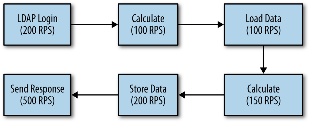
From a business perspective, the proprietary calculations are the most important thing; they are the reason the program exists, and the reason we are paid. Yet making them 100% faster will yield absolutely no benefit in this example. Any application (including a single, standalone JVM) can be modeled as a series of steps like this, where data flows out of a box (module, subsystem, etc.) at a rate determined by the efficiency of that box.^[5] Data flows into a subsystem at a rate determined by the output rate of the previous box.

Assume that an algorithmic improvement is made to the business calculation so that it can process 200 RPS, the load injected into the system is correspondingly increased. The LDAP system can handle the increased load: so far, so good, and 200 RPS will flow into the calculation module, which will output 200 RPS.

But the database can still process only 100 RPS. Even though 200 RPS flow into the database, only 100 RPS flow out of it and into the other modules. The total throughput of the system is still only 100 RPS, even though the efficiency of the business logic has doubled. Further attempts to improve the business logic will prove futile until time is spent improving the other aspects of the environment.

It’s not the case that the time spent optimizing the calculations in this example is entirely wasted: once effort is put into the bottlenecks elsewhere in the system, the performance benefit will finally be apparent. Rather, it is a matter of priorities: without testing the entire application, it is impossible to tell where spending time on performance work will pay off.

I work with the performance of both Java SE and EE, and each of those groups have a set of tests they characterize as microbenchmarks. To a Java SE engineer, that term connotes an example like that in the first section: the measurement of something quite small. Java EE engineers tend to use that term to apply to something else: benchmarks that measure one aspect of performance, but that still execute a lot of code.

An example of a Java EE “microbenchmark” might be something that measures how quickly the response from a simple JSP can be returned from an application server. The code involved in such a request is substantial compared to a traditional microbenchmark: there is a lot of socket-management code, code to read the request, code to find (and possibly compile) the JSP, code to write the answer, and so on. From a traditional standpoint, this is not microbenchmarking.

This kind of test is not a macrobenchmark either: there is no security (e.g., the user does not log into the application), no session management, and no use of a host of other Java EE features. Because it is only a subset of an actual application, it falls somewhere in the middle—it is a mesobenchmark. Mesobenchmarks are not limited to the Java EE arena: it is a term I use for benchmarks that do some real work, but are not full-fledged applications.

Mesobenchmarks have fewer pitfalls than microbenchmarks and are easier to work with than macrobenchmarks. It is unlikely that mesobenchmarks will contain a large amount of dead code that can be optimized away by the compiler (unless that dead code actually exists in the application, in which case optimizing it away is a good thing). Mesobenchmarks are more easily threaded: they are still more likely to encounter more synchronization bottlenecks than the code will encounter when run in a full application, but those bottlenecks are something the real application will eventually encounter on larger hardware systems under larger load.

Still, mesobenchmarks are not perfect. A developer who uses a benchmark like this to compare the performance of two application servers may be easily led astray. Consider the hypothetical response times of two application servers shown in Table 2-1.

The developer who uses only a simple JSP to compare the performance of the two servers might not realize that server two is automatically creating a session for each request. She may then conclude that server one will give her the fastest performance. Yet if her application always creates a session (which is typical), she will have made the incorrect choice, since it takes server one much longer to create a session.^[6]

Even so, mesobenchmarks offer a reasonable alternative to testing a full-scale application; their performance characteristics are much more closely-aligned to an actual application than are the performance characteristics of microbenchmarks. And there is of course a continuum here. A later section in this chapter presents the outline of a common application used for many of the examples in subsequent chapters. That application has an EE mode, but that mode doesn’t use session replication (high availability), nor the EE platform-based security, and though it can access an enterprise resource (i.e., a database), in most examples it just makes up random data. In SE mode, it mimics some actual (but quick) calculations, there is no GUI or user interaction occurring, nor anything else likely to be found in a real application.

Mesobenchmarks are also good for automated testing, particularly at the module level.

Many of the examples throughout the book are based on a sample application that calculates the “historical” high and low price of a stock over a range of dates, as well as the standard deviation during that time. Historical is in quotes here because in the application, all the data is fictional; the prices and the stock symbols are randomly generated.

The full source code for all examples in this book are online at www.oreilly.com, but this section covers basic points about the code. The basic object with in the application is a StockPrice object that represents the price range of a stock on a given day:

public interface StockPrice {
        String getSymbol();
        Date getDate();
        BigDecimal getClosingPrice();
        BigDecimal getHigh();
        BigDecimal getLow();
        BigDecimal getOpeningPrice();
        boolean isYearHigh();
        boolean isYearLow();
        Collection<? extends StockOptionPrice> getOptions();
}

The sample applications typically deal with a collection of these prices, representing the history of the stock over a period of a year (or 25 years, depending on the example):

public interface StockPriceHistory {
        StockPrice getPrice(Date d);
        Collection<StockPrice> getPrices(Date startDate, Date endDate);
        Map<Date, StockPrice> getAllEntries();
        Map<BigDecimal,ArrayList<Date>> getHistogram();
        BigDecimal getAveragePrice();
        Date getFirstDate();
        BigDecimal getHighPrice();
        Date getLastDate();
        BigDecimal getLowPrice();
        BigDecimal getStdDev();
        String getSymbol();
}

The basic implementation of this class loads a set of prices from the database:

public class StockPriceHistoryImpl implements StockPriceHistory {
    ...
    public StockPriceHistoryImpl(String s, Date startDate,
        Date endDate, EntityManager em) {
        Date curDate = new Date(startDate.getTime());
        symbol = s;
        while (!curDate.after(endDate)) {
            StockPriceImpl sp = em.find(StockPriceImpl.class,
                         new StockPricePK(s, (Date) curDate.clone()));
            if (sp != null) {
                Date d = (Date) curDate.clone();
                if (firstDate == null) {
                    firstDate = d;
                }
                prices.put(d, sp);
                lastDate = d;
            }
            curDate.setTime(curDate.getTime() + msPerDay);
        }
    }
    ...
}

The architecture of the samples is designed to be loaded from a database, and that functionality will be used in the examples in Chapter 11. However, for ease of running the examples, most of the time the examples will use a mock entity manager which generates random data for the series. In essence, most examples are module-level mesobenchmarks which are suitable for illustrating the performance issues at hand—but we would only have an idea of the actual performance of the application when the full application is run (as in Chapter 11).

One caveat is that a number of the examples are therefore dependent on the performance of the random number generator in use. Unlike the microbenchmark example, this is by design, as it allows the illustration of several performance issues in Java.^[7]

The examples are also heavily dependent on the performance of the BigDecimal class, which is used to store all the data points. This is a standard choice for storing currency data; if the currency data is stored as primitive double objects, then rounding of half-pennies and smaller amounts becomes quite problematic. From the perspective of writing examples, that choice is also useful as it allows some “business logic” or lengthy calculation to occur—particularly in calculating the standard deviation of a series of prices. The standard deviation relies on knowing the square root of a BigDecimal number. The standard Java API doesn’t supply such a routine, but the examples use this method:

    public static BigDecimal sqrtB(BigDecimal bd) {
        BigDecimal initial = bd;
        BigDecimal diff;
        do {
            BigDecimal sDivX = bd.divide(initial, 8, RoundingMode.FLOOR);
            BigDecimal sum = sDivX.add(initial);
            BigDecimal div = sum.divide(TWO, 8, RoundingMode.FLOOR);
            diff = div.subtract(initial).abs();
            diff.setScale(8, RoundingMode.FLOOR);
            initial = div;
        } while (diff.compareTo(error) > 0);
        return initial;
    }

This is an implementation of the Babylonian method for estimating the square root of a number. It isn’t the most efficient implementation; in particular, the initial guess could be much better, which would save some iterations. That is deliberate since it allows the calculation to take some time (emulating business logic), though it does illustrate the basic point made in Chapter 1: often the better way to have faster Java code is to write a better algorithm, independent of any Java tuning or Java coding practices that are employed.

The standard deviation, average price, and histogram of an implementation of the StockPriceHistory interface are all derived values. In different examples, these value will be calculated eagerly (when the data is loaded from the entity manager) or lazily (when the method to retrieve the data is called). Similarly, the StockPrice interface references a StockOptionPrice interface, which is the price of certain options for the given stock on the given day. Those option values can be retrieved from the entity manager either eagerly or lazily. In both cases, the definition of these interfaces allows these different approaches to be compared in different situations.

These interfaces also fit naturally into a Java EE application: a user can visit a JSP page that lets her enter the symbol and date range for a stock she is interested in. In the standard example, the request will go through the a standard servlet which parses the input parameters, calls a stateless EJB with an embedded JPA bean to get the underlying data, and forwards the response to a JSP page which formats the underlying data into an HTML presentation:

    protected void processRequest(HttpServletRequest request,
                        HttpServletResponse response)
                        throws ServletException, IOException {
        try {
            String symbol = request.getParameter("symbol");
            if (symbol == null) {
                symbol = StockPriceUtils.getRandomSymbol();
            }
            ... similar processing for date and other params...
            StockPriceHistory sph;
            DateFormat df = localDf.get();
            sph = stockSessionBean.getHistory(symbol, df.parse(startDate),
                            df.parse(endDate), doMock, impl);
            String saveSession = request.getParameter("save");
            if (saveSession != null) {
                .... Store the data in the user's session ....
                .... Optionally store the data in a global cache for
                .... use by other requests
            }
            if (request.getParameter("long") == null) {
                // Send back a page with about 4K of data
                request.getRequestDispatcher("history.jsp").
                        forward(request, response);
            }
            else {
                // Send back a page with about 100K of data
                request.getRequestDispatcher("longhistory.jsp").
                        forward(request, response);
            }
        }

This class can inject different implementations of the history bean (for eager or lazy initialization, among other things); it will optionally cache the data retrieved from the back end database (or mock entity manager). Those are the common options when dealing with the performance of an enterprise application (in particular, caching data in the middle tier is sometimes considered to be the big performance advantage of an application server). Examples throughout the book will examine those trade-offs as well.

The simplest way of measuring performance is to see how long it takes to accomplish a certain task: retrieve the history of 10,000 stocks for a 25-year period and calculate the standard deviation of those prices; produce a report of the payroll benefits for the 50,000 employees of a corporation; execute a loop 1,000,000 times.

In the non-Java world, this testing is straightforward: the application is written, and the time of its execution is measured. In the Java world, there is one wrinkle to this: just-in-time compilation. That process is described in Chapter 4; essentially it means that it takes a few minutes (or longer) for the code to be fully optimized and operate at peak performance. For that (and other) reasons, performance studies of Java are quite concerned about warm-up periods: performance is most often measured after the code in question has been executed long enough for it to have been compiled and optimized.

On the other hand, in many cases the performance of the application from start to finish is what matters. A report generator that processes 10,000 data elements will complete in a certain amount of time; to the end user, it doesn’t matter if the first 5,000 elements are processed 50% more slowly than the last 5,000 elements. And even in something like an application server—where the server’s performance will certainly improve over time—the initial performance matters. It may take 45 minutes for an application server to reach peak performance in certain configurations. To the users accessing the application during that time, the performance during the warm-up period does matter.

For those reasons, many examples in this book are batch-oriented (even if that is a little uncommon).

A throughput measurement is based on the amount of work that can be accomplished in a certain period of time. Although the most common examples of throughput measurements involve a server processing data fed by a client, that is not strictly necessary: a single, standalone application can measure throughput just as easily as it measures elapsed time.

In a client-server test, a throughput measurement means that clients have no think time. If there is a single client, that client sends a request to the server. When it receives a response, it immediately sends a new request. That process continues; at the end of the test, the client reports the total number of operations it achieved. Typically, the client has multiple threads doing the same thing, and the throughput is the aggregate measure of the number of operations all clients achieved. Usually this number is reported as the number of operations per second, rather than the total number of operations over the measurement period. This measurement is frequently referred to as transactions per second (TPS), requests per second (RPS), or operations per second (OPS).

All client-server tests run the risk that the client cannot send data quickly enough to the server. This may occur because there aren’t enough CPU cycles in the client machine to run the desired number of client threads, or because the client has to spend a lot of time processing the request before it can send a new request. In those cases, the test is effectively measuring the client performance rather than the server performance, which is usually not the goal.

This risk depends on the amount of work that each client thread performs (and the size and configuration of the client machine). A zero think-time (throughput-oriented) test is more likely to encounter this situation, since each client thread is performing a lot of work. Hence, throughput tests are typically executed with fewer client threads (less load) than a corresponding test that measures response time.

It is common for tests that measure throughput to report also the average response time of its requests. That is an interesting piece of information, but changes in that number aren’t indicative of a performance problem unless the reported throughput is the same. A server that can sustain 500 operations per second with a 0.5 second response time is performing better than a server than reports a 0.3 second response time but only 400 operations per second.

Throughput measurements are almost always taken after a suitable warmup period, particularly since what is being measured is not a fixed set of work.

The last common test is one that measures response time: the length of time it takes between sending a request from a client until the response is received.

The difference between a response time test and a throughput test (assuming the latter is client-server based) is that client threads in a response-time test sleep for some period of time between operations. This time is referred to as think time. A response time test is designed to mimic more closely what a user does: she enters a URL in a browser, spends some time reading the page that comes back, clicks on a link in the page, spends some time reading that page, and so on.

When think time is introduced into a test, throughput becomes fixed: a given number of clients executing requests with a given think time will always yield the same TPS (with some slight variance; see sidebar). At that point, the important measurement is the response time for the request: the effectiveness of the server is based on how quickly it responds to that fixed load.

while (!done) {
    time = executeOperation();
    Thread.currentThread().sleep(30*1000);
}

while (!done) {
    time = executeOperation();
    Thread.currentThread().sleep(30*1000 - time);
}

There are two ways of measuring response time. Response time can be reported as an average: the individual times are added together and divided by the number of requests. Response time can also be reported as a percentile request, for example the 90th% response time. If 90% of responses are less than 1.5 seconds and 10% of responses are greater than 1.5 seconds, then 1.5 seconds is the 90th% response time.

One difference between the two numbers is in the way outliers affect the calculation of the average—since they are included part of the average, large outliers will have a large effect on the average response time.

Figure 2-2 shows a graph of 20 requests with a somewhat typical range for response times. The response times range from 1 to 5 seconds. The average response time (represented by the lower heavy line along the X-axis) is 2.35 seconds, and 90% of the responses occur in 4 or less seconds (represented by the upper heavy line along the X-axis).

Figure 2-2. Typical Set of Response Times

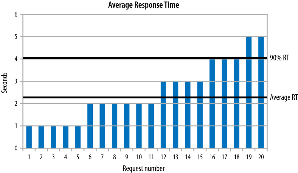
This is the usual scenario for a well-behaved test. Outliers can skew that analysis, as the data in Figure 2-3 shows.

Figure 2-3. Set of Response Times with an Outlier

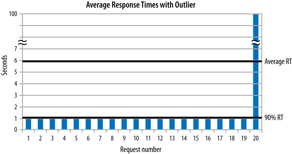
This data set includes a huge outlier: one request took 100 seconds. As a result, the positions of the 90th% and average response times are reversed. The average response time is a whopping 5.95 seconds, but the 90th% response time is 1.0 seconds. Focus in this case should be given to reducing the effect of the outlier (which will drive down the average response time).

Outliers like that are rare in general, though they can more easily occur in Java applications because of the pause times introduced by garbage collection.^[8] In performance testing, the usual focus is on the 90th% response time (or sometimes the 95th% or 99th% response time; there is nothing magical about 90%). If you can only focus on one number, a percentile-based number is the better choice, since achieving a smaller number there will benefit a majority of users. But it is even better to look at both the average response time and at least one percentile-based response time, so that you do not miss the case where there are large outliers.

% fhb -W 1000 -r 300/300/60 -c 25  http://host:port/StockServlet?stock=SDO
ops/sec: 8.247
% errors: 0.0
avg. time: 0.022
max time: 0.045
90th %: 0.030
95th %: 0.035
99th %: 0.035