
Chapter 3. A Java Performance Toolbox
Performance analysis is all about visibility—knowing what is going on inside of an application, and in the application’s environment. Visibility is all about tools. And so performance tuning is all about tools.
In Chapter 2, I stressed the importance of taking a data-driven approach to performance: you must measure the application’s performance and understand what those measurements mean. Performance analysis must be similarly data-driven: you must have data about what, exactly, the program is doing in order to make it perform better. How to obtain and understand that data is the subject of this chapter.
There are hundreds of tools that provide information about what a Java application is doing, and of course it is impractical to look at all of them. Many of the most important tools come with the JDK or are developed in open source at java.net, and even though those tools have other open source and commercial competitors, this chapter focuses mostly on the JDK tools as a matter of expedience.
Operating System Tools and Analysis
The starting point for program analysis is actually not Java-specific at
all: it is the basic set of monitoring tools that come with the
operating system. On Unix-based systems, these are sar (System Accounting
Report) and its constituent tools like
vmstat
+iostat,
+prstat,
and so on.
On Windows, there are graphical
resource monitors as well as command-line utilities like
typeperf.
Whenever performance tests are run, data should be gathered from the operating system. At a minimum, information on cpu, memory, and disk usage should be collected; if the program uses the network, information on network usage should be gathered as well. If performance tests are automated, this means relying on command-line tools (even on Windows)—but even if tests are running interactively, it is better to have a command-line tool that captures output, rather than eyeballing a GUI graph and guessing what it means. The output can always be graphed later when doing analysis.
CPU Usage
Let’s look first at monitoring the CPU and what it tells us about Java programs. CPU usage is typically divided into two categories: user time, and system time (Windows refers to this as privileged time). User time is the percentage of time the CPU is executing application code, while system time is the percentage of time the CPU is executing kernel code. System time is related to the application; if the application performs I/O, for example, the kernel will execute the code to read the file from disk, or write the network buffer, and so on. Anything that uses an underlying system resource will cause the application to use more system time.
The goal in performance is to drive CPU usage as high as possible for as short a time as possible. That may sound a little counter-intuitive; you’ve doubtless sat at your desktop and watched it struggle because the CPU is 100% utilized. So let’s consider what the CPU usage actually tells us.
The first thing to keep in mind is that the CPU usage number is an average over an interval—5 seconds, 30 seconds, perhaps even as little as 1 second (though never really less than that). Say that the average CPU usage of a program is 50% for the 10 minutes it takes to execute. If the code is tuned such that the CPU usage goes to 100%, the performance of the program will double: it will run in 5 minutes. If performance is doubled again, the CPU will still be at 100% during the 2.5 minutes it takes the program to complete. The CPU number is an indication of how effectively the program is using the CPU, and so the higher the number the better.
If I run
vmstat 1 on
my Linux desktop, I will get a series of lines (one every second)
that look like this:
% vmstat 1
procs -----------memory---------- ---swap-- -----io---- -system-- ----cpu----
 r  b   swpd   free   buff  cache   si   so    bi    bo   in   cs us sy id wa
 2  0      0 1797836 1229068 1508276 0    0     0     9 2250 3634 41  3 55  0
 2  0      0 1801772 1229076 1508284 0    0     0     8 2304 3683 43  3 54  0
 1  0      0 1813552 1229084 1508284 0    0     3    22 2354 3896 42  3 55  0
 1  0      0 1819628 1229092 1508292 0    0     0    84 2418 3998 43  2 55  0
This example comes from running an application with one active thread—that makes the example easier to follow, but the concepts apply even if there are multiple threads.
During each second, the CPU is busy for 450 milliseconds (42% of the time executing user code, and 3% of the time executing system code). Similarly, the CPU is idle for 550 milliseconds. The CPU can be idle for a number of reasons:
- The application might be blocked on a synchronization primitive and unable to execute until that lock is released.
- The application might be waiting for something, such as a response to come back from a call to the database.
- The application might have nothing to do.
These first two situations are always indicative of something which can be addressed. If contention on the lock can be reduced, or the database can be tuned so that it sends the answer back more quickly, then the program will run faster and the average CPU use of the application will go up (assuming, of course, that there isn’t another such issue that will continue to block the application).
That third point is where confusion often lies. If the application has something to do (and it is not prevented from doing it because it is waiting for a lock or another resource), then the CPU will spend cycles executing the application code. This is a general principle, not specific to Java. Say that you write a simple script containing an infinite loop. When that script is executed, it will consume 100% of a CPU. The following batch job will do just that in Windows:
ECHO OFF
:BEGIN
ECHO LOOPING
GOTO BEGIN
REM We never get here...
ECHO DONE
Consider what it would mean if this script did not consume 100% of a CPU. It would mean that the operating system had something it could do—it could print yet another line saying LOOPING—but it chose instead to be idle. Being idle doesn’t help anyone in that case, and if we were doing a useful (lengthy) calculation, forcing the CPU to be periodically idle would mean that it would take longer to get the answer we are after.
If you run this command on a single CPU machine, much of the time you are unlikely to notice that it is running. But if you attempt to start a new program, or time the performance of another application, then you will certainly see the effect. Operating systems are good at time-slicing programs that are competing for CPU cycles, but there will be less CPU available for the new program, and it will run more slowly. That experience sometimes leads people to think it would be a good idea to leave some idle CPU cycles just in case something else needs them.
But the operating system cannot guess what you want to do next; it will (by default) execute everything it can rather than leaving the CPU idle.
Java and Single-CPU usage
To return to the discussion of the Java application—what does periodic, idle CPU mean in that case? It depends on the type of application. If the code in question is a batch-style application where there is a fixed amount of work, you should never see idle CPU because there is no work to do. Driving the CPU usage higher is always the goal for batch jobs, because it means the job will be completed faster. If the CPU is already at 100%, then you can of course still look for optimizations that allow the work to be completed faster (while trying also to keep the CPU at 100%).
If the measurement involves a server-style application that accepts requests
from
some source, then there may be idle time because no work is available:
e.g., when a web server has processed all outstanding HTTP requests and is
waiting
for the next request.
This is where the average time comes in. The sample
vmstat
output was taken during execution of an application server that was receiving
one request every second.
Ut took 450 milliseconds for
the application server to process that request—meaning that the CPU was actually 100% busy for
450 milliseconds, and 0% busy for 550 milliseconds. That was reported as the
CPU being 45% busy.
Although it usually happens at a level of granularity that is too small to visualize, the expected behavior of the CPU when running a load-based application is to operate in short bursts like this. The same macro-level pattern will be seen from the reporting if the CPU received one request every half-second and the average time to process the request was 225 milliseconds. The CPU would be busy for 225 milliseconds, idle for 275 milliseconds, busy again for 225 milliseconds, and idle for 275 milliseconds: on average, 45% busy and 55% idle.
If the application is optimized so that each request takes only 400 milliseconds, then the overall CPU usage will also be reduced (to 40%). This is the only case where driving the CPU usage lower makes sense—when there is a fixed amount of load coming into the system and the application is not constrained by external resources. On the other hand, that optimization also gives you the opportunity to add more load into the system, ultimately increasing the CPU utilization. And at a micro-level, optimizing in this case is still a matter of getting the CPU usage to 100% for a short period of time (the 400 milliseconds it takes to execute the request)—it’s just that the duration of the CPU spike is too short to effectively register as 100% using most tools.
Java and Multi-CPU usage
This example has assumed a single thread running on a single CPU, but the concepts are the same in the general case of multiple threads running on multiple CPUs. Multiple threads can skew the average of the CPU in interesting ways—one such example is shown in Chapter 5, which shows the effect of the multiple GC threads on CPU usage. But in general, the goal for multiple threads on a multi-CPU machine is still to drive the CPU higher by making sure individual threads are not blocked, or to drive the CPU lower (over a long interval) because the threads have completed their work and are waiting for more work.
In a multi-threaded, multi-CPU case, there is one important addition regarding when CPUs could be idle: CPUs can be idle even when there is work to do. This occurs if there are no threads available in the program to handle that work. The typical case here is an application with a fixed-size thread pool which is running various tasks. Each thread can execute only one task at a time, and if that particular task blocks (e.g., waiting for a response from the database), the thread cannot pick up a new task to execute in the meantime. Hence, there can be periods where there are tasks to be executed (work to be done), but no thread available to execute them; the result is some idle CPU time.
In that example, the size of the thread pool should be increased. However, don’t assume that just because idle CPU is available, it means that the size of the thread pool should be increased in order to accomplish more work. The program may not be getting CPU cycles for the other two reasons previously mentioned—because of bottlenecks in locks or external resources. It is important to understand why the program isn’t getting CPU before determining a course of action.[10]
Looking at the CPU usage is a first step in understanding application performance, but it is only that: use it to see if the code is using all the CPU that can be expected, or if it points to some synchronization or resource issue.
The CPU Run Queue
Both Windows and Unix systems allow you to monitor the number of threads
that are able to run (meaning that they are not blocked on I/O, or sleeping,
and so on). Unix systems refer to this as the run queue, and several tools
include the run queue length in their output. That includes the
vmstat
output
in the last section: the first number in each line is the length of the
run queue. Windows refers to this number as the processor queue, and
reports it (among other ways) via
typeperf:
C:> typeperf -si 1 "SystemProcessor Queue Length"
"05/11/2013 19:09:42.678","0.000000"
"05/11/2013 19:09:43.678","0.000000"
There is a very important difference in the output here: the run queue length
number
on Unix system (which was either one or two in the sample
vmstat output) is
the number of all
threads that are running or that could run if there were an available CPU.
In that example, there was always at least one thread
that wanted to run: the single thread doing application work. Hence, the run
queue length was always at least one. Keep in mind that
the run queue length represents everything on the machine, so sometimes
there are other threads
(from completely separate processes) that want to run, which is why the run
queue length sometimes was two in that sample output.
In Windows, the processor queue length does not include the number of threads
that are currently running. Hence, in the
typeperf
sample output, the
processor queue number was zero, even though the machine was running the
same single-threaded
application with one thread always executing.
If there are more threads to run than available CPUs, performance will begin to degrade. In general, then, you want the processor queue length to be 0 on Windows, and equal to (or less than) the number of CPUs on Unix systems. That isn’t a hard and fast rule; there are system processes and other things that will come along periodically and briefly raise that value without any significant performance impact. But if the run queue length is too high for any significant period of time, it is an indication that the machine is overloaded and you should look into reducing the amount of work the machine is doing (either by moving jobs to another machine, or optimizing the code).
Quick Summary
- CPU time is the first thing to examine when looking at performance of an application.
- The goal in optimizing code is to drive the CPU usage up (for a shorter period of time), not down.
- Understand why CPU usage is low before diving in and attempting to tune an application.
Disk Usage
Monitoring disk usage has two important goals. The first of these regards the application itself: if the application is doing a lot of disk I/O, then it is easy for that I/O to become a bottleneck.
Knowing when disk I/O is a bottleneck is tricky, because it depends on the behavior of the application. If the application is not efficiently buffering the data it writes to disk (an example of which is in Chapter 12), the disk I/O statistics will be quite low. But if the application is performing more I/O than the disk can handle, the disk I/O statistics will be quite high. In either situation, performance can be improved; be on the lookout for both.
The basic I/O monitors on some systems are better than on others. Here is
some partial output of
iostat
on a Linux system:
% iostat -xm 5
avg-cpu:  %user   %nice %system %iowait  %steal   %idle
          23.45    0.00   37.89    0.10    0.00   38.56

          Device:         rrqm/s   wrqm/s     r/s     w/s    rMB/s
          sda               0.00    11.60    0.60   24.20     0.02

          wMB/s avgrq-sz avgqu-sz   await r_await w_await  svctm  %util
          0.14    13.35     0.15    6.06    5.33    6.08   0.42   1.04
The application here is writing data to disk sda. At first glance, the
disk statistics look good. The w_await—which is the time to service each
I/O write—is fairly low (6.08 milliseconds), and the disk is only 1.04%
utilized.[11] But there is a clue here that something is wrong: the system is
spending 37.89% of its time in the kernel. If the system is doing other
I/O (in other programs), that’s one thing; if all that system time
is from the application being tested,
then something inefficient is happening.
The fact that the system is doing 24.2 writes per second is another clue here: that is a lot of writes when writing only 0.14 MB per second. I/O has become a bottleneck; we can now look into how the application is performing its writes
The other side of the coin comes if the disk cannot keep up with the I/O requests:
% iostat -xm 5
avg-cpu:  %user   %nice %system %iowait  %steal   %idle
          35.05    0.00    7.85   47.89    0.00    9.20

          Device:         rrqm/s   wrqm/s     r/s     w/s    rMB/s
          sda               0.00     0.20    1.00  163.40     0.00

          wMB/s avgrq-sz avgqu-sz   await r_await w_await  svctm  %util
          81.09  1010.19   142.74  866.47   97.60  871.17   6.08 100.00
The nice thing about Linux is that it tells us immediately that the disk is
100% utilized; it also tells us that processes are spending 47.89% of their
time in
iowait
(that is, waiting for the disk).
Even on other systems where only raw data is available, that data will tell
us something is amiss: the time to complete the I/O (w_await) is 871
milliseconds, the queue size is quite large, and the disk is writing
81 MB of data/second. This all points to disk I/O as a
problem, and that
the amount of I/O in the application (or,
possibly, elsewhere in the system) must be reduced.
A second reason to monitor disk usage—even if the application is not expected to perform a significant amount of I/O—is to help monitor if the system is swapping. Computers have a fixed amount of physical memory, but they can run a set of applications that use a much larger amount of virtual memory. Applications tend to reserve more memory than they actually need, and they usually operate on only a subset of their memory. In both cases, the operating system can keep the unused parts of memory on disk, and page it into physical memory only if it is needed.
For the most part, this kind of memory management works well, especially for interactive and GUI programs (which is good, or your laptop would require much more memory than it has). It works less well for server-based applications, since those applications tend to use more of their memory. And it works particularly badly for any kind of Java application (including a Swing-based GUI application running on your desktop) because of the Java heap. More details about that appear in Chapter 5.
A system that is swapping—moving pages of data from main memory to
disk and vice versa—will have generally bad performance. Other system
tools can also report if the system is swapping; for example, the
vmstat
output has two columns (si, for swap in, and so,
for swap out) that alert us if the system is swapping. Disk activity is
another indicator that swapping might be occurring.
Quick Summary
- Monitoring disk usage is important for all applications. For applications that don’t directly write to disk, system swapping can still affect their performance.
- Applications that write to disk can be bottlenecked both because they are writing data inefficiently (too little throughput) or because they are writing too much data (too much throughput).
Network Usage
If you are running an application that uses the network—for example, a Java EE application server—then you must monitor the network traffic as well. Network usage is similar to disk traffic: the application might be inefficiently using the network so that bandwidth is too low, or the total amount of data written to a particular network interface might be more than the interface is able to handle.
Unfortunately, standard system tools are less than ideal for monitoring network traffic because they typically show only the number of packets and number of bytes that are sent and received over a particular network interface. That is useful information, but it doesn’t tell us if the network is under- or over-utilized.
On Unix systems, the basic network monitoring tool is
netstat
(and on most
Linux distributions,
netstat
is not even included and must be obtained
separately). On Windows,
typeperf
can be used in scripts to monitor
the network usage—but here is a case where the GUI has an advantage: the
standard Windows resource monitor will display a graph showing what percentage
of the network is in use. Unfortunately, the GUI is of little help in an automated
performance testing scenario.
Fortunately, there are many open-source and commercial tools that
monitor network bandwidth. On Unix systems, one popular command-line
tool is
nicstat
(http://sourceforge.net/projects/nicstat), which presents
a summary of the traffic on each interface, including the degree to which the
interface is utilized:
% nicstat 5
Time      Int       rKB/s   wKB/s   rPk/s   wPk/s   rAvs    wAvs   %Util  Sat
17:05:17  e1000g1   225.7   176.2   905.0   922.5   255.4   195.6  0.33   0.00
The e1000g1 interface is a 1000 MB interface; it is not utilized very
much (0.33%)
in this example. The usefulness of this tool—and others like it—is that it calucates the utilization of the interface. In this output,
there is 225.7 KB/sec of data being written and 176.2 KB/sec of data being read
over the interface.
Doing the division for a 1000 MB
network yields the 0.33% utilization figure, and the
nicstat
tool was able
to figure out the bandwidth of the interface automatically.
Tools such as
typeperf
or
netstat
will report the amount of data read and written,
but to figure out the network utilization, you must determine the bandwidth
of the interface and
perform the calculation in your own scripts. Be careful that the bandwidth
is measured in bits per second, but tools generally report bytes per second.
A 1000 megabit network yields 125 megabytes per second. In this example,
0.22 megabytes per second are read and 0.16 megabytes per second are written;
adding those and dividing by 125 yields a 0.33% utilization rate. So there
is no magic to
nicstat
(or similar) tools; they are just more
convenient to use.
Networks cannot sustain a 100% utilization rate. For local-area Ethernet networks, a sustained utilization rate over 40% indicates that the interface is saturated. If the network is packet-switched or utilizes a different medium, the maximum possible sustained rate will be different; consult a network architect to determine the appropriate goal. This goal is independent of Java, which will simply utilize the networking parameters and interfaces of the operating system.
Quick Summary
- For network-based applications, make sure to monitor the network to make sure it hasn’t become a bottleneck.
- Applications that write to the network can be bottlenecked both because they are writing data inefficiently (too little throughput) or because they are writing too much data (too much throughput).
Java Monitoring Tools
To gain insight into the JVM itself, Java monitoring tools are required. There are a number of tools that come with the JDK:
-
jcmd Print basic class, thread, and VM information of a Java process. This is suitable for use in scripts; it is executed like this:
%
jcmd process_id command optional_argumentsSupplying the command
helpwill list all possible commands, and supplyinghelp <command>will give the syntax for a particular command.-
jconsole - Provides a graphical view of JVM activities, including thread usage, class usage, and GC activities
-
jhat - Reads and helps analyze memory heap dumps. This is a post-processing utility.
-
jmap - Provides heap dumps and other information about JVM memory usage. Suitable for scripting, though the heap dumps must be used in a post-processing tool.
-
jinfo - Provides visibility into the system properties of the JVM, and allows some system properties to be set dynamically. Suitable for scripting.
-
jstack - Dumps the stacks of a Java process. Suitable for scripting.
-
jstat - Provides information about GC and class loading activities. Suitable for scripting.
-
jvisualvm -
A GUI tool to monitor a JVM, profile a running application, and analyze JVM heap dumps (which is a post-processing activity, though
jvisualvmcan also take the heap dump from a live program).
These tools fits into these broad areas:
- Basic VM information
- Thread information
- Class information
- Live GC analysis
- Heap Dump post-processing
- Profiling a JVM
As you likely noticed, there is not a one-to-one mapping here; many tools perform functions in multiple areas. So rather than exploring each tool individually, we’ll take a look at the functional areas of visibility that are important to Java, and discuss how various tools provide that information. Along the way, we’ll discuss other tools (some open-source, some commercial) that provide the same basic functionality but which have advantages over the basic JDK tools.
Basic VM information
JVM tools can provide basic information about a running JVM process: how long it has been up, what JVM flags are in use, JVM system properties, and so on.
- uptime
- The length of time the JVM has been up can be found via this command:
% jcmd process_id VM.uptime
- System properties
-
The set of items in the
System.getProperties()can be displayed with either of these commands:
%jcmd process_id VM.system_propertiesor %jinfo -sysprops process_id
This includes all properties set on the command line with a -D option,
any properties dynamically added by the application, and the set of
default properties for the VMpe.
- JVM Version
- The version of the VM is obtained like this:
% jcmd process_id VM.version
- JVM Command Line
-
The command line can be displayed in the VM summary tab of
jconsole, or viajcmd:
% jcmd process_id VM.command_line
- JVM Tuning Flags
- The tuning flags in effect for an application can be obtained like this:
% jcmd process_id VM.flags [-all]
Working with tuning flags
There are a lot of tuning flags that can be given to a VM, and many of those
flags are a major focus of this book. Keeping track of those flags and their
default values can be a little daunting; those last two examples of jcmd are
quite useful in that regard. The
command_line
command shows
which flags were specified directly on the command line. The flags
command shows which flags were set on the command line, plus
some flags that were set directly by the VM (because their value
was determined ergonomically). Including the -all option lists every
flag within the JVM.
There are hundreds of JVM tunings flags,
and most of them are very
obscure; it is recommended that most of them never be changed (see sidebar).
Figuring out which flags are in effect is a frequent task when diagnosing
performance issues, and the jcmd commands can do that for a running JVM.
Often, what you’d rather figure out is what the platform-specific defaults
for a particular JVM are, in which case using the
-XX:+PrintFlagsFinal
option on the command line is more useful.
A useful way to determine what the flags are set to on a particular platform is to execute this command:
% java other_options -XX:+PrintFlagsFinal -version
...Hundreds of lines of output, including...
uintx InitialHeapSize                          := 4169431040     {product}
intx InlineSmallCode                           = 2000            {pd product}
You should include all other options in the command line because some options
affect others, particularly when setting GC-related flags.
This will print out the entire list of VM flags and their values (the same
as is printed via the VM.flags -all option to jcmd for a live JVM).
Flag data from these commands is printed in one of the two ways shown. The colon in the first line of included output indicates that a non-default value is in use for the flag in question. This can happen for the following reasons:
- The flag’s value was specified directly on the command-line.
- Some other option indirectly changed that option.
- The VM calculated the default value ergonomically.
The second line (without a colon) indicates that value is the default
value for this version of the JVM. Default values for some flags
may be different
on different platforms—which is shown in the final column of this
output.
product
means that the default setting of
the flag is uniform across all platforms; pd product indicates that the
default setting of the flag is platform dependent.
Other possible values for
the last column include
manageable
(the flag’s value can be changed
dynamically during runtime) and
C2 diagnostic
(the flag provides diagnostic
output for the compiler engineers to understand how the compiler is
functioning).
Yet another way to see this information for a running applications is with
jinfo—but the advantage to jinfo is that it allows certain flag values
to be changed during execution of the program.
Here is how to retrieve the values of all the flags in the process:
% jinfo -flags process_id
With the -flags option, jinfo will provide information about all flags;
otherwise it prints only those specified on the command line. The output
from either of these commands isn’t as easy to read as that of the
-XX:+PrintFlagsFinal
option, but jinfo has other features to keep in mind.
jinfo can inspect the value of an
individual flag:
% jinfo -flag PrintGCDetails process_id
-XX:+PrintGCDetails
Although jinfo does not itself indicate if a flag is manageable or not,
flags that are manageable (as identified when using the
PrintFlagsFinal
argument) can be turned on or off via jinfo:
%jinfo -flag -PrintGCDetails process_id# turns off PrintGCDetails %jinfo -flag PrintGCDetails process_id-XX:-PrintGCDetails
Be aware that jinfo can change the value of any flag, but that doesn’t
mean that the JVM will respond to that change.
For example, most flags that affect the behavior of a garbage collection
algorithm are used at startup time to determine various ways that the collector
will behave.
Altering a flag later via jinfo does not cause
the JVM to change its behavior; it will continue executing based on
how the algorithm was initialized. So this technique only works for those
flags marked
manageable
in the output of the
PrintFlagsFinal
command.
Quick Summary
-
jcmdcan be used to find the basic VM information—include the value of all the tuning flags—for a running application. -
Default flag values can be found by including
-XX:+PrintFlagsFinalon a command line. This is useful for determining the default ergonomic settings of flags on a particular platform. -
jinfois useful for inspecting (and in some cases changing) individual flags.
Thread Information
jconsole and jvisualvm display information (in real-time) about the
number of threads
running in an application.
It can be very useful to look at the stack of running threads to determine
if they are blocked. The stacks can be obtained via jstack:
% jstack process_id
... Lots of output showing each thread's stack ...
Stack information can also be obtained from jcmd:
% jcmd process_id Thread.print
... Lots of output showing each thread's stack ...
See Chapter 9 for more details on monitoring thread stacks.
Class Information
Information about the number of classes in use by an application can be
obtained from jconsole or jstat. jstat can also provide
information about class compilation.
See Chapter 12 for more details on class usage by applications, and Chapter 4 for details on monitoring class compilation.
Live GC Analysis
Virtually every monitoring tool reports something about GC activity.
jconsole displays live graphs of the heap usage; jcmd allows
GC operations to be performed; jmap can print heap summaries, information
on the permanent generation, or create a heap dump; and jstat produces a lot
of different views of what the garbage collector is doing.
See Chapter 5 for examples of how these programs monitor GC activities.
Heap Dump Post Processing
Heap dumps can be captured from the jvisualvm GUI, or from the command line
using jcmd or jmap. The heap dump is a snapshot
of the heap that can be analyzed with various tools, including jvisualvm
and jhat. Heap dump processing is one area where third-party tools have
traditionally been a step ahead of what comes with the JDK, so
Chapter 7 uses a third-party tool—the Eclipse Memory Analyzer
Tool—to provide examples of how to post-process heap dumps.
Profiling Tools
Profiliers are the most important tool in a performance analyst’s toolbox. There are many profilers available for Java, each with its own advantages and disadvantages. Profiling is one area where it often makes sense to use different tools—particularly if they are sampling profilers. One sampling profiler may find different problems than another one, even on the same application.
Almost all Java profiling tools are themselves written in Java and work by “attaching” themselves to the application to be profiled—meaning that the profiler opens a socket (or other communication channel) to the target application. The target application and the profiling tool then exchange information about the behavior of the target application.
This means you must pay attention to tuning the profiling tool just as you would tune any other Java application. In particular, if the application being profiled is large, it will transfer quite a lot of data to the profiling tool, so the profiling tool must have a sufficiently large heap to handle the data. It is often a good idea to run the profiling tool with a concurrent GC algorithm as well; ill-timed full GC pauses in the profiling tool can cause the buffers holding the data to overflow.
Sampling Profilers
Profiling happens in one of two modes: sampling mode or instrumented mode. Sampling mode is the basic mode of profiling and carries the least amount of overhead. That’s important, since one of pitfalls of profiling is that by introducing measurement into the application, you are altering its performance characteristics.[12] Limiting the impact of profiling will lead to results that more closely model how the application behaves under usual circumstances.
Unfortunately, sampling profilers can be subject to all sorts of errors. Sampling profilers work when a timer periodically fires; the profiler then looks at each thread and determines which method the thread is executing. That method is then charged with having been executed since the timer previously fired.
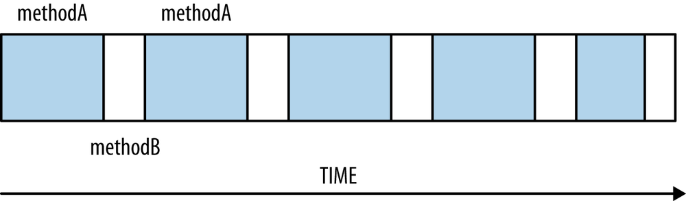
The most common sampling error is illustrated by Figure 3-1. The
thread here is alternating between executing
methodA
(shown in the shaded
bars) and
methodB
(shown in the clear bars). If
the timer fires only when the thread happens to be in
methodB,
the profile
will report that the thread spent all its time executing
methodB;
in
reality, more time was actually spent in
methodA.
This is the most common sampling error, but it is by no means the only one. The way to minimize these errors is to profile over a longer period of time, and to reduce the time interval between samples. Reducing the interval between samples is counter-productive to the goal of minimizing the impact of profiling on the application; there is a balance here. Profiling tools resolve that balance differently, which is one reason why one profiling tool may happen to report much different data than a different tool.
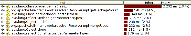
Figure 3-2 shows a basic sampling profile taken to measure the
startup of a domain of the GlassFish application server. The profile shows
that the bulk of the time (19%) was spent in the
defineClass1()
method,
followed by the
getPackageSourcesInternal()
method, and so on. It isn’t a
surprise that the startup of a program would be dominated by the
performance of defining classes; in order to make this code faster,
the performance of class loading must be improved.
Note carefully the last statement: it is the performance of class loading that
must be improved, and not the performance of the
defineClass1()
method.
The common assumption when looking at a profile is that improvements
must come from optimizing the top method in the profile. However, that is
often too limiting an approach. In this case, the
defineClass1()
method is
part of the JDK, and a native method at that; its performance isn’t going to
be improved without rewriting the JVM. Still, assume
that it could be re-written so that it took 60% less time.
That will translate to a 10% overall improvement in the execution time—which is certainly nothing to sneeze at.
More commonly, though, the top method in a profile may take 2% of 3% of total time; cutting its time in half (which is usually enormously difficult) will only speed up application performance by 1%. Focusing only on the top method in a profile isn’t usually going to lead to huge gains in performance.
Instead, the top method(s) in a profile should point you to the area in which to search for optimizations. GlassFish performance engineers aren’t going to attempt to make class definition faster, but they can figure out how to make class loading in general be faster—by loading fewer classes, or loading classes in parallel, and so on.
Quick Summary
- Sampling-based profilers are the most common profiler.
- Because of their relatively low profile, sampling profilers introduce fewer measurement artifacts into a profile.
- Different sampling profiles behave differently; each may be better for a particular application.
Instrumented Profilers
Instrumented profilers are much more intrusive than sampling profilers, but they can also give more beneficial information about what’s happening inside the program. Figure 3-3 uses the same profiling tool to look at startup of the same GlassFish domain, but this time it is using instrumented mode.
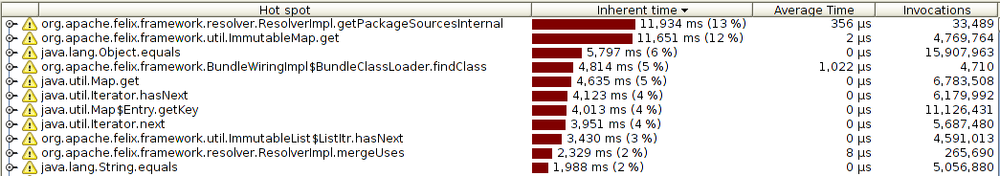
A few things are immediately apparent about this profile. First, notice that
the “hot” method is now
getPackageSourcesInternal(),
accounting for 13% of
the total time (not 4%, as in the previous example). There are other
expensive methods near the top of the profile, and the
defineClass1()
method
doesn’t appear at all. The tool also now reports the number of times each
method was invoked, and it calculates the average time per invocation
based on that number.
Is this a better profile than the sampled version? It depends; there is
no way to know in a given situation which is the more accurate profile.
The invocation count of an instrumented profile is certainly accurate, and
that additional information is often quite helpful in determining where the
code is actually spending more time and which things are more fruitful to
optimize. In this case, although the
ImmutableMap.get()
method is consuming
12% of the total time, it is called 4.7 million times. We can have a much
greater performance by impact reducing the total number of calls to
this method rather than speeding up
its implementation.
On the other hand, instrumented profilers work by altering the bytecode sequence of classes as they are loaded (inserting code to count the invocations and so on). They are much more likely to introduce performance differences into the application than are sampling profilers. For example, the JVM will inline small methods (see Chapter 4) so that no method invocation is needed when the small method code is executed. The compiler makes that decision based on the size of the code; depending on how the code is instrumented, it may no longer be eligible to be inlined. This may cause the instrumented profiler to overestimate the contribution of certain methods. And inlining is just one example of a decision that the compiler makes based on the layout of the code; in general, the more the code is instrumented (changed), the more likely that its execution profile will change.
There is also an interesting technical reason why the
ImmutableMap.get()
method shows up in this profile and not the sampling profile. Sampling
profilers in Java can only take the sample of a thread when the thread is
at a safepoint—essentially, whenever it is allocating memory. The
get()
method may never arrive at a safepoint and so may never get sampled. That
means the sampling profile can underestimate the contribution of that method
to the program execution.
In this example, both the instrumented and sampled profiles pointed to the same general area of the code: class loading and resolution. In practice, it is possible for different profilers to point to completely different areas of the code. Profilers are good estimators, but they are only making estimates: some of them will be wrong some of the time.
Quick Summary
- Instrumented profilers yield more information about an application, but can possibly have a greater effect on the application than a sampling profiler.
- Instrumented profilers should be set up to instrument small sections of the code—a few classes or packages. That limits their impact on the application’s performance.
Blocking Methods and Thread Timelines
Figure 3-4 shows the GlassFish startup using a different
instrumented profiling tool (the NetBeans profiler). Now the execution
time is dominated by the
park()
and
parkNanos()
methods (and to a lesser extent, the
read()
method).
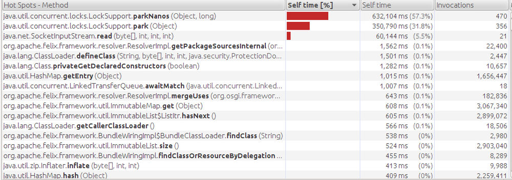
Those methods (and similar blocking methods) do not consume CPU time, so
they are not contributing to the overall CPU usage of the application.
Their execution cannot necessarily be optimized. Threads in the application are
not spending 632 seconds executing code in the
parkNanos()
method; they are
spending 632 seconds waiting for something else to happen (e.g.,
for another thread to call the
notify()
method). The same is true
of the park() and read() methods.
For that reason, most profilers will not report methods that are blocked; those threads are shown as being idle (and in this case, NetBeans was set to explicitly include those and all other Java-level methods). In this particular example, that is a good thing: the threads that are parked are the threads of the Java threadpool that will execute servlet (and other) requests as they come into the server. No such requests occur during startup, and so those threads remain blocked—waiting for some task to execute. That is their normal state.
In other cases, you do want to see the time spent in those blocking calls.
The time that a thread spends inside the
wait()
method—waiting for
some other thread to notify it—is a significant determinant of the overall
execution time of many applications. Most Java-based profilers have filter
sets and other options that can be tweaked to show or hide these blocking
calls.
Alternately, it is usually more fruitful to examine the execution patterns of threads rather than the amount of time a profiler attributes to the blocking method itself. Figure 3-5 shows such a thread display from the Oracle Solaris Studio profiling tool.
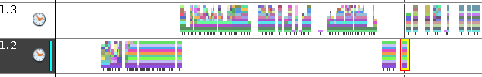
Each horizontal area here is a different thread (so there are two threads in the figure: thread 1.3 and thread 1.2). The colored (or different gray-scale) bars represent execution of different methods; blank areas represent places where the thread is not executing. At a high level, observe that thread 1.2 executed a lot of code and then waited for thread 1.3 to do something; thread 1.3 then waited a bit of time for thread 1.2 to do something else, and so on. Diving into those areas with the tool lets us learn how those threads are interacting with each other.
Notice too that there are blank areas where no thread appears to be
executing. The image shows only two of many threads in the application, so
it is possible that these threads are waiting for one of those other threads
to do something, or the thread could be
executing a blocking read() (or similar) call.
Quick Summary
- Threads that are blocked may or may not be a source of a performance issue; it is necessary to examine why they are blocked.
- Blocked threads can be identified by the method that is blocking, or by a timeline analysis of the thread.
Native Profilers
Native profiling tools are those that profile the JVM itself. This allows visibility into what the JVM is doing, and if an application includes its own native libraries, it allows visibility into that code as well. Any native profiling tool can be used to profile the C code of the JVM (and of any native libraries), but some native-based tools can profile both the Java and C/C++ code of an application.
Figure 3-6 shows the now-familiar profile from starting GlassFish in the Oracle Solaris Studio analyzer tool, which is a native profiler that understands both Java and C/C++ code.[13]
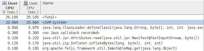
The first difference to note here is that there is a total of 25.1 seconds
of CPU time recorded by the application, and 20 seconds of that is in
JVM-System.
That is the code attributable to the JVM itself—the JVM’s compiler threads
and garbage collection threads (plus a few other ancillary threads).
We can
drill into that further; in this case, we’d see that virtually all of
that time is spent by
the compiler (as is expected during startup, when there is a lot of code
to compile).
A very small amount of time is spent by
the garbage collection threads in this example.
Unless the goal is to hack on the JVM itself, that native visibility is enough, though if we wanted, we could look into the actual JVM functions and go optimize them. But the key piece of information from this tool—one that isn’t available from a Java-based tool—is the amount of time the application is spending in garbage collection. In Java profiling tools, the impact of the garbage collection threads is nowhere to be found.[14]
Once the impact of the native code has been examined, it can be filtered out to focus on the actual startup (Figure 3-7).
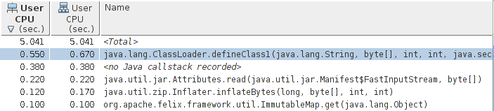
Once again, the sampling profiler here points to the
defineClass1()
method
as the hottest method, though the actual time spent in that method and
its children—0.67 seconds out of 5.041 seconds—is about 11% (significantly
less than the last sample-based profiler reported). This profile also points
to some additional things to examine: reading and unzipping jar files.
As these are related to class loading, we were on the right track for those
anyway—but in this case it is interesting to see that the actual I/O
for reading the jar files (via the
inflateBytes()
method) is a few percentage
points. Other tools didn’t show us that—partly because the native code
involved in the Java zip libraries got treated as a blocking call and was
filtered out.
No matter which profiling tool—or better yet, tools—you use, it is quite important to become familiar with their idiosyncrasies. Profilers are the most important tool to guide the search for performance bottlenecks, but you must learn to use them to guide you to areas of the code to optimize, rather than looking focusing solely on the top hot spot.
Quick Summary
- Native profilers provide visibility into both the JVM code and the application code.
- If a native profiler shows that time in garbage collection dominates the CPU usage, then tuning the collector is the right thing to do. If it shows significant time in the compilation threads, however, that is usually not affecting the application’s performance.
Java Mission Control
The commercial releases of Java 7 (starting with 7u40) and Java 8 include a new monitoring and control feature called Java Mission Control. This feature will be familiar to users of JDK 6-based JRockit JVMs (where the technology originated), since it is part of Oracle’s merging of technologies for Java 7. Mission Control is not part of the open-source development of Java and is available only with a commercial license (i.e., the same procedure as for competitive monitoring and profiling tools from other companies).
The Java Mission Control program (jmc) starts a window that displays
the JVM processes on the machine and lets you select one or more processes to
monitor. Figure 3-8 shows mission control monitoring an instance
of the GlassFish application server.
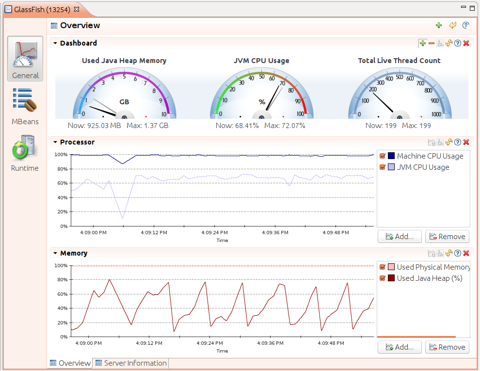
This display shows basic information that mission control is monitoring: CPU usage and heap usage. Note, though, that the CPU graph includes the total CPU on the machine (which is essentially 100%, even though the application being monitored here is using only about 70%). That is a key feature of the monitoring: mission control has the ability to monitor the entire system, not just the JVM that has been selected. The upper dashboard can be configured to display JVM information (all kinds of statistics about garbage collection, class loading, thread usage, heap usage, and so on) as well as OS-specific information (total machine CPU and memory usage, swapping, load averages, and so on).
Like other monitoring tools, mission control can make JMX calls into whatever mbeans the application has available.
Java Flight Recorder
The key feature of mission control is the Java Flight Recorder (JFR). As its name suggests, JFR data is a history of events in the JVM that can be used to diagnose the past performance and operations of the JVM.
The basic operation of JFR is that some set of events are enabled (for example, one event is that a thread is blocked waiting for a lock). Each time a selected event occurs, data about that event is saved (either in memory or to a file). The data stream is held in a circular buffer, so only the most recent events are available. Mission control can then display those events—either taken from a live JVM or read from a saved file—and you can perform analysis on those events to diagnose performance issues.
All of that—the kind of events, the size of the circular buffer, where
it is stored and so on—are controlled via various arguments to the JVM,
via the mission control GUI, and by jcmd commands as the program runs. By
default, JFR is set up so that it has very low overhead—an impact
below 1% of the program’s performance. That overhead will change as
more events are enabled, or the threshold at which events are reported is
changed,
and so on.
The details of all that configuration are discussed later in this section,
but first we’ll examine
what the display of these events look like, since that makes it easier
to understand how JFR works.
JFR Overview
This example uses a JFR recording taken from a GlassFish application server over a six-minute period. The server is running the stock servlet discussed in Chapter 2. As the recording is loaded into mission control, the first thing it displays is a basic monitoring overview (Figure 3-9):
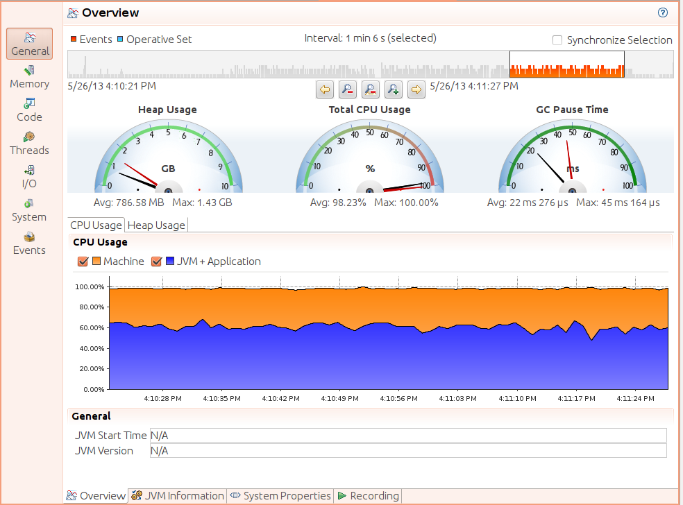
This display is quite similar to what mission control displays when doing basic monitoring. Above the gauges showing CPU and heap usage, there is a timeline of events (represented by a series of vertical bars). The timeline allows us to zoom into a particular region of interest; although in this example the recording was taken over a six-minute period, I zoomed into a 1 minute 6 second interval near the end of the recording.
The graph here for CPU usage is a little clearer as to what is going on; the GlassFish JVM is the bottom portion of the graph (averaging about 70% usage), and the machine is running at 100% CPU usage. Along the bottom, there are some other tabs to explore: information about system properties and how the JFR recording was actually made. The icons that run down the left-hand side of the window are more interesting: those icons provide visibility into the application behavior.
JFR Memory View
The information gathered here is extensive. Figure 3-10 shows just one panel of the Memory view.
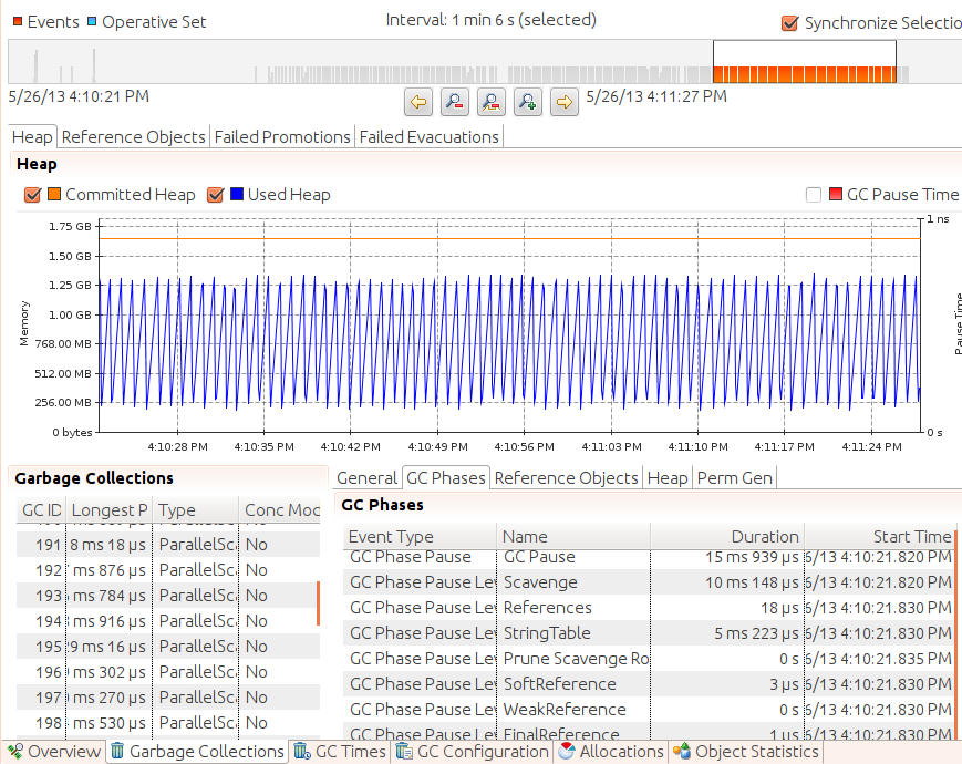
The graph here shows that memory is fluctuating fairly regularly as the
young generation is cleared (and interestingly enough, there is no overall
growth of the heap in this application: nothing is promoted to the old
generation). The lower-left panel shows all the collections that occurred
during the recording, including their duration and what kind of collection
they were (always a
ParallelScavenge
in this example). When one of those events is
selected, the bottom-right panel breaks that down even further, showing all
the specific phases of that collection and how long each took.
As can be seen from the various tabs on this page, there is a wealth of other available information: how long and how many reference objects were cleared, whether there are promotion or evacuation failures from the concurrent collectors, the configuration of the GC algorithm itself (including the sizes of the generations and the survivor space configurations), and even information on the specific kinds of objects that were allocated. As you read through Chapter 5 and Chapter 6, keep in mind how this tool can diagnose the problems that are discussed there. If you need to understand why CMS bailed out and performed a full GC (was it due to promotion failure?), or how the JVM has adjusted the tenuring threshold, or virtually any other piece of data about how and why GC behaved as it did, JFR will be able to tell you.
JFR Code View
The Code page in mission control shows basic profiling information from the recording (Figure 3-11).
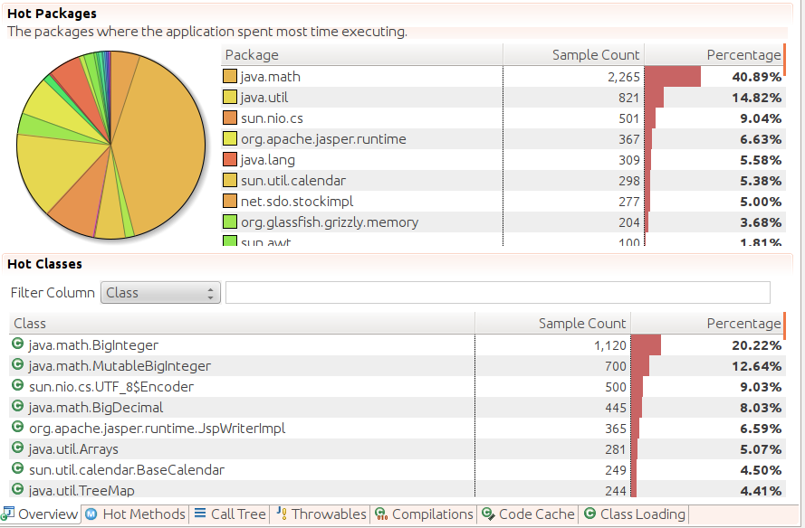
The first tab on this page shows an aggregation by package name, which is
an interesting feature not found in many profilers; unsurprisingly, the
stock application spends 41% of its time doing calculations in the
java.math package. At the bottom, there are other tabs for the traditional
profile views: the hot methods and call tree of the profiled code.
Unlike other profilers, flight recorder offers other modes of visibility into the code. The “Throwables” tab provides a view into the exception processing of the application (Chapter 12 has a discussion of why excessive exception processing can be bad for performance). There are also tabs that provide information on what the compiler is doing, including a view into the code cache (see Chapter 4).
There are other displays like this—for threads, I/O, and system events—but for the most part, these displays simply provide nice views into the actual events in the JFR recording.
Overview of JFR Events
JFR produces a stream of events which are saved as a recording. The displays seen so far provide views of those events, but the most powerful way to look at the events is on the event panel itself, as seen in Figure 3-12.
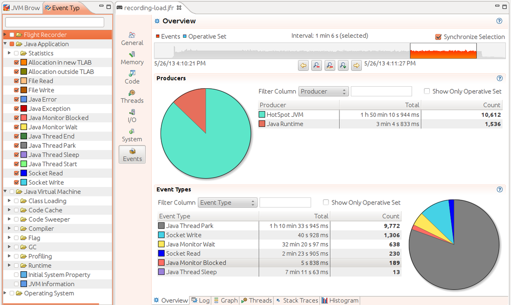
The events to display can be filtered in the left-hand panel of this window; here, only the application-level events are selected. Be aware that when the recording is made, only certain kinds of events are included in the first place—at this point, we are doing post-processing filtering (the next section will show how to filter the events included in the recording).
Within the 66 second interval in this example, the application produced 10,612 events from the JVM and 1,536 events from the JDK libraries, and the six event types generated in that period are shown near the bottom of the window. I’ve already discussed why the thread park and monitor wait events for this example will be high; those can be ignored (and in fact they are often a good candidate to filter out). What about the other events?
Over the 66 second period, multiple threads in the application spent 40
seconds writing to sockets. That’s not an unreasonable number for an
application server running across four CPUs (i.e., with 264 seconds of
available time), but it does indicate that
performance could be improved by writing less data to the clients (using
the techniques outlined in Chapter 10.) Similarly, multiple threads spent 143
seconds reading from sockets. That number sounds worse, and it is worthwhile
looking at the traces involved with those events, but it turns out that
there are several threads that use blocking I/O to read administrative
requests which are expected to arrive periodically. In between those
requests—for long periods of time—the threads sit blocked on the read()
method. So the read time here turns out to be acceptable—just as when
using a profiler, it is up to you to determine whether a lot of
threads blocked in I/O is expected, or if it indicates a performance issue.
That leaves the monitor blocked events. As discussed in Chapter 9, contention for locks goes through two levels: first the thread spins waiting for the lock, and then it uses (in a process call lock inflation) some CPU- and OS-specific code to wait for the lock. A standard profiler can give hints about that situation, since the spinning time is included in the CPU time charged to a method. A native profiler can give some information about the locks subject to inflation, but that can be hit-or-miss (e.g., the Oracle Studio analyzer does a very good job of that on Solaris, but Linux lacks the operating system hooks necessary to provide the same information). The JVM, though, can provide all this data directly to JFR.
An example using lock visibility is shown in Chapter 9, but the general take away about JFR events is that—since they come directly from the JVM—they offer a level of visibility into an application that no other tool can provide. In Java 7u40, there are 77 event types that can be monitored with JFR. The exact number and types of events will vary slightly depending on release, but here are some of the more useful ones.
The list of events that follows displays two bullet points for each
event type.
Events
can collect basic information that can be collected with other tools like
jconsole and jcmd; that kind of information is described in the first
bullet. The second bullet describes information the event provides which
is difficult to obtain outside of JFR.
- Class Loading
- Number of classes loaded and unloaded
- Which classloader loaded the class; time required to load an individual class
- Thread Statistics
- Number of threads created and destroyed; thread dumps
- Which threads are blocked on locks (and the specific lock they are blocked on)
- Throwables
- Throwable classes used by the application
- How many exceptions and errors are thrown and the stack trace of their creation
- TLAB Allocation
- The number of allocations in the heap and size of TLABs
- The specific objects allocated in the heap and the stack trace where they are allocated
- File and Socket I/O
- Time spent performing I/O
- Time spent per read/write call, the specific file or socket taking a long time to read or write
- Monitor Blocked
- Threads waiting for a monitor
- Specific threads blocked on specific monitors and the length of time they are blocked
- Code Cache
- Size of code cache and how much it contains
- Methods removed from the code cache; code cache configuration
- Code Compilation
- Which methods are compiled, OSR compilation, and length of time to compile
- Nothing specific to JFR, but unifies information from several sources
- Garbage Collection
- Times for GC, including individual phases; sizes of generations
- Nothing specific to JFR, but unifies the information from several tools
- Profiling
- Instrumenting and sampling profiles
- The JFR sampling profiler is a good first-pass profiling tool but lacks the full features of a true profiler
Enabling JFR
In the commercial version of the Oracle JVM, JFR is initially disabled. To enable
it, add the flags
-XX:+UnlockCommercialFeatures
-XX:+FlightRecorder
to
the command line of the application. This enables JFR as a feature, but no
recordings
will be made until the recording process itself is enabled. That can occur
either through a GUI, or via the command line.
Enabling JFR via Mission Control
The easiest way to enable recording is through Java Mission Control GUI (jmc).
When jmc is started, it displays a list of all the JVM processes running
on the current system. The JVM processes are displayed in a tree-node
configuration; expand the node under the “Flight Recorder” label to bring
up the flight recorder window shown in Figure 3-13.
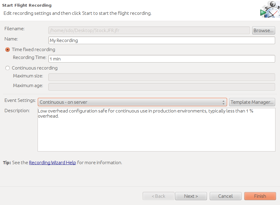
Flight recordings are made in one of two modes: either for a fixed duration (1 minute in this case), or continuously. For continuous recordings, a circular buffer is utilized; the buffer will contain the most recent events that are within the desired duration and size.
To perform proactive analysis—meaning that you will start a recording and then generate some work, or start a recording during a load testing experiment after the JVM has warmed up—then a fixed duration recording should be used. That recording will give a good indication of how the JVM responded during the test.
The continuous recording is best for reactive analysis. This lets the JVM keep the most recent events, and then dump out a recording in response to some event. For example, the WebLogic application server can trigger that a recording be dumped out in response to an abnormal event in the application server (such as a request that takes more than five minutes to process). You can set up your own monitoring tools to dump out the recording in response to any sort of event.
Enabling JFR via the command line
After enabling JFR (with the
-XX:+FlightRecorder
option), there are two
ways to control how and when the actual recording should happen.
The recording parameters can be controlled when the JVM starts by using
the
-XX:+FlightRecorderOptions=string
parameter; this is most useful
for reactive recordings. The string in that parameter is a list of
comma-separated name-value pairs taken from these options:
- name=name
- The name used to identify the recording.
-
defaultrecording=
<true|false> -
Whether to start the recording initially. The default value is
false; for reactive analysis, this should be set totrue. - settings=path
- Name of the file containing the JFR settings (see next section).
-
delay=
time -
The amount of time (e.g.
30s,1h) before the recording should start. -
duration=
time - The amount of time to make the recording.
- filename=path
- Name of the file to write the recording to.
-
compress=
<true|false> -
Whether to compress (with gzip) the recording; the default is
false. -
maxage=
time - Maximum time to keep recorded data in the circular buffer.
-
maxsize=
size -
Maximum size (e.g.,
1024K,1M) of the recording’s circular buffer.
Setting up a default recording like that can be useful in some circumstances,
but for more flexibility, all options can be controlled with jcmd during a run
(assuming that the
-XX:+FlightRecorder
option was specified in the first
place).
To start a flight recording:
% jcmd process_id JFR.start [options_list]
The options list is a series of comma-separated
name=value
pairs that
control how the recording is made. The possible options are exactly the
same as those which can be specified on the command line to the
-XX:+FlightRecorderOptions=string
flag.
If a continuous recording has been enabled, the current data in the circular buffer can be dumped to a file at any time via this command:
% jcmd process_id JFR.dump [options_list]
where the list of options includes:
- name=name
- The name under which the recording was started.
- recording=n
-
The number of the JFR recording (see the next example for
JFR.check). - filename=path
- The location to dump the file to.
It is possible that multiple JFR recordings have been enabled for a given process. To see the available recordings:
% jcmd process_id JFR.check [verbose]
Recordings in this case are identified by the name used to begin them, as well as an arbitrary recording number (which can be used in other JFR commands).
Finally, to abort a recording in process:
% jcmd process_id JFR.stop [options_list]
That command takes the following options:
- name=name
- The recording name to stop.
- recording=n
-
The recording number (from
JFR.check) to stop. - discard=boolean
-
If
true, discard the data rather than writing it to the previously-provided filename (if any). - filename=path
- Write the data to the given path.
In an automated performance testing system, running these command-line tools and producing a recording is useful when it comes time to examine those runs for regressions.
Selecting JFR events
JFR (presently) supports approximately 77 events. Many of these events
are periodic events: they occur every few milliseconds (e.g., the profiling
events work on a sampling basis). Other events are triggered only when the
duration of the event exceeds some threshold (e.g., the event for reading a
file is triggered only if the read() method has taken more than some
specified amount of time).
Collecting events naturally involves some overhead. The threshold at which events are collected—since it increases the number of events—also plays a role in the overhead that comes from enabling a JFR recording. In the default recording, not all events are collected (the six most-expensive events are not enabled), and the threshold for the time-based events is somewhat high. This keeps the overhead of the default recording to less than 1%.
There are times when extra overhead is worthwhile. Looking at TLAB events, for example, can help you determine if objects are being allocated directly to the old generation, but those events are not enabled in the default recording. Similarly, the profiling events are enabled in the default recording, but only every 20 milliseconds—that gives a good overview, but it can also lead to sampling errors.
The events (and the threshold for events) that JFR captures are defined in
a template (which is selected via the
settings
option on the command line).
JFR ships
with two templates: the default template (limiting events
so that the overhead will be less than 1%) and a profile template (which
sets most threshold-based events to be triggered every 10ms). The estimated
overhead of the profiling template is 2% (though, as always, your mileage
may vary, and
I typically observe a much lower overhead than that).
Templates are managed by the jmc template manager; you may have noticed a
button to start the template manager in Figure 3-13. Templates are
stored in two locations: under the $HOME/.jmc/<release> directory (local
to a user) and in the $JAVA_HOME/jre/lib/jfr directory (global for a JVM).
The template manager allows you to select a global template (the template
will say that it is “on server”), select a local template, or define a new
template. To define a template, cycle through the available events,
and enable (or disable) them as desired, optionally setting the threshold
at which the event kicks in.
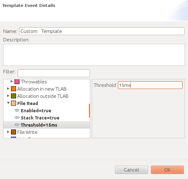
Figure 3-14 shows that the File Read event is enabled with a threshold of 15ms: file reads that take longer than that will cause an event to be triggered. This event has also been configured to generate a stack trace for the file read events. That increases the overhead—which in turn is why taking a stack trace for events is a configurable option.
The event templates are simple XML files, so the best way to determine which events are enabled in a template (and their thresholds and stack-trace configurations) is to read the XML file. Using an XML file also allows the local template file to be defined on one machine and then copied to the global template directory for use by others in the team.
Quick Summary
- Java Flight Recorder provides the best-possible visibility into the JVM, since it is built into the JVM itself.
- Like all tools, JFR involves some level of overhead into an application. For routine use, JFR can be enabled to gather a substantial amount of information with low overhead.
- JFR is useful in performance analysis, but it is also useful when enabled on a production system so that you can examine the events that led up to a failure.
Summary
Good tools are key to good performance analysis; in this chapter, we’ve just scratched the surface of what tools can tell us. The key things to keep in mind are:
- No tool is perfect, and competing tools have relative strengths. Profiler X may be a good fit for many applications, but there will always be cases where it misses something that Profiler Y points out quite clearly. Always be flexible in your approach.
- Command-line monitoring tools can gather important data automatically; be sure to include the gathering of this monitoring data in your automated performance testing.
- Tools rapidly evolve: some of the tools mentioned in this chapter are probably already obsolete (or at least have been superseded by new, superior tools). This is one area where it is important to keep up-to-date.
[11] The acceptable values for that depend on the physical disk, but the 5200 RPM disk in my desktop system behaves well when the service time is under 15 ms.
[12] Still, you must profile: how else will you know if the cat inside your program is still alive?
[13] Although it has Solaris in its name, this tool works on Linux systems as well; in fact, these images are from profiling on a Linux OS. However, the kernel architecture of Solaris allows the tool to provide even more application visibility when run on Solaris.
[14] Unless the test is run on a machine which is CPU-bound, the large amount of time in the compiler thread will not matter: that thread will consume a lot of one CPU on the machine, but as long as there are more CPUs available, the application itself won’t be impacted, since the compilation happens in the background.