6 Real-World DAQ Programming Techniques

In this section, we will cover LabVIEW programming techniques that are especially helpful for DAQ programming. The following areas will be addressed:

1.   Programming Structure for DAQ

2.   Analog Waveform Analysis

3.   File I/O for DAQ

4.   Averaging

5.   Speed and Efficiency

6.   Display Techniques

7.   Alarms

8.   Power Losses

6.1 PROGRAMMING STRUCTURE FOR DAQ

This section is applicable to many types of LabVIEW programming, but is specifically tailored for DAQ.

6.1.1 Handling Large Projects

Suppose you’re building a really large LabVIEW application, and you run into the usual problem of having many items cluttering your block diagrams with too many wires strewn about. Sound familiar? If not, you have not yet tried to build a really large LabVIEW application. Here’s a quick summary of tips for managing such large LabVIEW projects (also useful for small ones!):

1.   MOST IMPORTANT TIP: For your main White Loop, as most LabVIEW programs have, construct the loop with a single shift register containing a typedef custom control we’ll call the state cluster (described soon) containing all your data that may be used in subVIs.

2.   Cluster multiple controls or indicators on your front panel whenever it helps; this reduces the number of terminals on the block diagram.

3.   Avoid complex wiring on your block diagrams, and for this purpose, avoid crossing wires wherever possible.

4.   Avoid overlapping objects on your block diagrams.

5.   Restrict your block diagrams to 800 × 600 pixels if there’s any chance they will ever be viewed on other monitors. See Appendix E, item 7 for more details.

6.   Add comments to your block diagrams describing the “big picture”—a high-level description of what’s happening. Use these sparingly. I recommend coloring them all the same color; yellow or another light color is ideal for printing. I will not use such comments in this book, because I’m trying to keep my block diagrams simple.

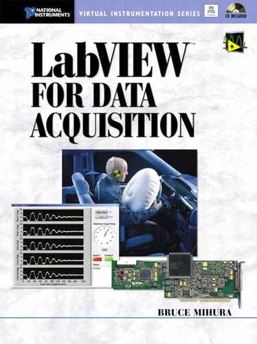
Now, let’s demonstrate these tips (do not follow along in LabVIEW, until we create the typedef custom control). Figure 6–1 shows an example of not following tips 2 and 3.

Figure 6–1
A working but sloppy VI–too many shift registers.

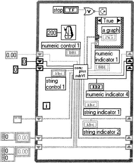
Ouch! This hurts my eyes just looking at it. I can simplify this greatly by combining my shift registers into one, as suggested by tip 1; see Figure 6–2.

Ahh—this is much easier on the eyes. Before I describe the typedef business of tip 1, let’s apply tip 3. This involves creating clusters of controls and clusters of indicators on the front panel, so as to simplify the block diagram, as shown in Figure 6–3.

As you can see, I’ve created one front panel cluster for most of the controls, and one for most of the indicators. For cosmetic or logical reasons, you may not want to combine all of your front panel objects as such, but bundle them into clusters whenever you can. I could have also included the stop button in the controls cluster, then dragged the Not Or function inside the subVI, but I usually prefer to leave it visible for high-level clarity. I have also not included my graph with the indicators, for two reasons:

Figure 6–2
Greatly improved from Figure 6–1—only one shift register.

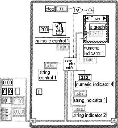
Figure 6–3
Improved even further from Figure 6–2—clustered controls and indicators.

1.   Most people like the looks of a graph by itself, not in a cluster.

2.   I now have control over the update rate of the graph, as it’s in the Case Structure (I may want to update it only at certain times, as a large graph can take a long time to draw).

Now let’s cover the typedef issue. The mechanics of creating a typedef are rather involved, so don’t be swamped by all of these tedious steps—once you know how to create a typedef, it’s not so hard.

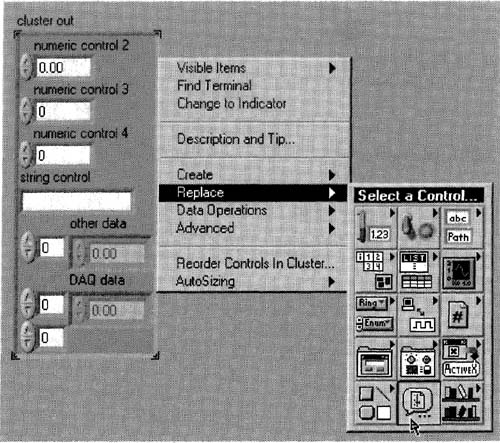
So what is a typedef, and why should you want one? Suppose you spend a fair amount of time modifying a control (or indicator) to look and behave just the way you want, and you want to save it because you think you’ll use it again. A typedef allows you to change just one saved instance of this control, and the others will automatically change themselves to match the saved one. For example, do you see where the wire from the shift register enters the subVI in the block diagram of Figure 6–3? Figure 6–4 shows what the front panel of that subVI might look like, and the wire connected to the calling VI’s shift register is connected to the cluster in and cluster out terminals.

Figure 6–4
Front panel objects illustrating the need for the typedef.

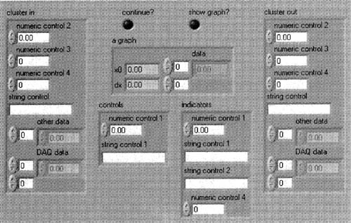
The exact same cluster type is used in the constant of the block diagram of Figure 6–3. That’s three separate places, just in this simple example, where the same typedef can be used. Your complex LabVIEW projets will often benefit by using a typedef as such to synchronize the data type of a cluster when it is being used by many sub VIs.

To create a typedef, we must first create a custom control, which is a front panel object that we customize to our application, then save to disk, usually with a .ctl file extension. A typedef is a particular type of custom control—we will create one shortly. A strict typedef is like a typedef, but it updates cosmetic properties like color and size, as well as data type, of the control wherever it’s being used.

Start following along in LabVIEW now.

Figure 6–5
Preparing to customize a front panel control.

1.   Create a new VI with a cluster control containing the items shown in Figure 6–6, or whatever you want in the cluster. In general, you should label all of your cluster’s elements, so you can manipulate them by name later on. Copy the control and change the copy to an indicator, then label the two cluster objects cluster in and cluster out, as shown in Figure 6–4.

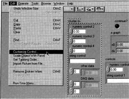
2.   To change this cluster control into a typedef, select the cluster control from your front panel, then select the Edit»Customize Control… menu item white the cluster control is selected; see Figure 6–5.
Once you select this menu item, up pops the control editor, shown in Figure 6–6, featuring your control (you can do some serious cosmetic surgery here, but that’s not the point of this book).

Figure 6–6
A front panel control, ready to be customized.

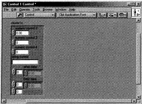
      You can now save this control as a custom control, much like you save a VI. Our custom control will soon be saved as a file with .ctl extension, not the usual .vi extension.

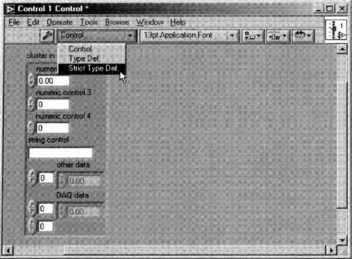
3.   Pop up on the Type Def. Status ring from the tool bar (which should say “Control” at first), then select the Strict Type Def. item, as shown in Figure 6–7.

Figure 6–7
Selecting this option, “Strict Type Def.”, will force the control to not only take on the same data type, but the same graphical look wherever it’s used on any front panel.

4.   Save this custom control as Cluster.ctl.I recommend giving it an icon, but this is not quite as important for custom controls as it is for subVIs, as custom controls’ icons are never seen in block diagrams. Their icons are seen in LabVIEW’s hierarchy window, however.

5.   Close this control editor—when asked to replace the original control, say yes. In the front panel from which this control came, the cluster in has just been replaced with this strict typedef control, but the cluster out indicator has not. So pop up on the cluster out control, and replace it with your recently saved Cluster. ctl, as in Figure 6–8.

Figure 6–8
A file dialog box will pop up once you select this item, from which you can select your custom control (Cluster .ctl), thus replacing cluster out with your typedef.

Why is this typedef so special? If you use it in all your subVIs that use this cluster, and you want to change them all at once, you can do so automatically and quickly by (1) opening the typedef custom control, (2) modifying it, (3) saving it, then (4) closing it. You must execute all four of these steps before all instances of this typedef will automatically update.

A couple of final tips in this section: When using your cluster typedef in subVIs as a state cluster, use the Unbundle By Name function to pick out the elements by name, and use the Bundle By Name function to modify the elements. For this to work, you must label any cluster elements you want to use in your typedef. Also, if you have one of these typedefs on a front panel and you want to quickly edit it, even if you’ve forgotten its file name, just pop up on the typedef and select Open Type Def.

One word of warning—when you increase the height or width of a strict typedef cluster control, and all of its instances are updated, many unseen instances of the typedef may overlap nearby front panel controls. To remedy this situation, it is convenient to place your strict typedef cluster controls such that they may grow vertically, but not horizontally, without overlapping other front panel objects, as shown in the front panel of Figure 6–4.

6.1.2 State Machines

If you have an electrical engineering degree from a college, or if you’re some sort of self-educated digital designer, chances are you’ve heard of a state machine. If not, this term is used to describe a process that is always in one state or another.

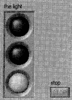
A simple example, shown in Figure 6–9, is a traffic light, which has three basic states—green, yellow, and red.

Figure 6–9
A traffic light showing a green light (please pretend to see a green light on the bottom in this black and white book).

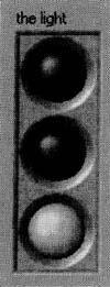
Figure 6–9 is really a cluster of three Booleans on a LabVIEW front panel that I’ve created to look something like a traffic light. I’ve colored the True states of the Booleans green, yellow, and red, from bottom to top. I’ve colored all the False states black.

Figure 6–10 presents a graphical way to think of this state machine (with just one traffic light), supposing we have a really speedy light.

Figure 6–10
Our first state machine.

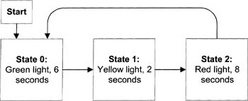
Real traffic lights had better not be this fast, but we’ll build a fast one in LabVIEW so you don’t get bored waiting for the light to change!

To implement a state machine in LabVIEW, simply use a Case Structure inside a White Loop, then add an integer in a shift register to cycle through the states. We cannot have a long delay inside any of these LabVIEW states, because we must respond to user events quickly. We should only stay in any given state for a split second. So, let’s reconsider a slightly more complex state machine for our single traffic light that doesn’t linger in any one state for very long. To do this, you could consider the traffic light as a state machine having six states: (0) green, (1) changing from green to yellow, (2) yellow, (3) changing from yellow to red, (4) red, and (5) changing from red to green, as illustrated in Figure 6–11.

Figure 6–11
A useful rendition of our first state machine, based on Figure 6–10.

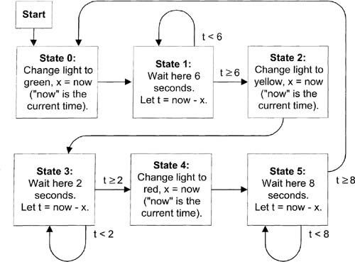
LabVIEW has the ability to get the current time in seconds, via its Get Date/Time In Seconds function . For example, I just ran this function, and it returned 3039173669.54, which is the number of seconds since some specific time in 1904, as its Help window indicates. The x, now, and t variables in the diagram use this function to calculate delay times white waiting for a light to change—if this variable business is clear to you, skip the next paragraph.

Start with State 0. The light is changed to green, and the current time is recorded as x by the statement x = now. Let’s pretend the current time is 10.0 (it will really be a much larger number, but we’ll use small numbers here for simplicity), so the statement x = now means that x is now 10. The x, now, and t are variables, or storage spaces, for numbers. In this state machine, x always records the time just before we begin a delay. We then move to State 1; now, as always, is the current time. Supposing our main loop occurs every 0.2 seconds, now is now 10.2, so t = now - x is now 0.2. Effectively, in State 1, t tells you how long you’ve been in State 1. If you have been in State 1 less than 6 seconds, t > 6 is True, so the t > 6 arrow indicates that you return to State 1. Once you’ve been in State 1 for 6 seconds or more, t ≥ 6 is True, so you proceed to State 2, which will change the light to yellow. The same logic that applies for States 0 and 1 also applies for States 2 and 3, as well as States 4 and 5.

Whenever we’re delaying for a light, we’re really quickly looping back into the same state, as is usually happening in states 1, 3, and 5 in Figure 6–11.

Let’s build this traffic light state machine in LabVIEW. Although we won’t be directly using the DAQ Vis, the timing concepts herein are applicable to many DAQ applications. Create the following VI, using these tips:

1.   Create a cluster of three Boolean indicators on the front panel, such as the traffic light shown in Figure 6–9. If you don’t want to go to the trouble of coloring them, just label any three Booleans as green, yellow, and red, and drop them into a cluster on the front panel. If you do want to create this beautiful cluster control, the Boolean indicators are the Round LED found in the Controls »Boolean palette—make sure that their colored states correspond to True, and their black states correspond to False (this can be tricky). In any event, the cluster order is such that green is cluster element 0, yellow is 1, and red is 2. Also drop the standard Stop Button from the Controls»Boolean palette, as shown in Figure 6–12.

Figure 6–12
The front panel of our VI, with a cluster of three Booleans trying to imitate a traffic light.

2.   You can quickly create the block diagram constant the light (the cluster of three Booleans inside the state cluster) by popping up on the terminal of the light, and selecting Create»Constant.

3.   Start by building the partially complete VI as shown in Figure 6–13, wiring the unseen Case 1 just like Case 0. Make sure x has DBL representation, as SGL would not be able to represent time.

Figure 6–13
We begin to build a “state machine” VI.

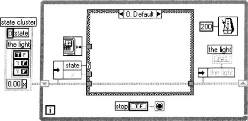
      Notice that you must label the three cluster elements, state, the light, and x, for their names to appear in the Unbundle By Name functions. I have not shown case 1 in the illustration, but it’s wired just like case 0 for now.

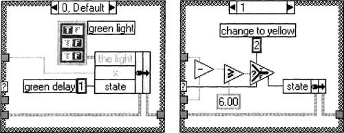
4.   We will set up the Case Structure cases 0 to 5 to directly correspond to states 0 to 5 in the state machine diagram in Figure 6–11. Create states 0 and 1 in cases 0 and 1 of Case Structure, as in Figure 6–14.

5.   Since we need two more cases similar to case 0, and two more similar to case 1, duplicate each of these cases twice—we want a total of three cases similar to case 0 and three cases similar to case 1. To duplicate a case, pop up on the wall of the Case Structure and select Duplicate Case.

      The more proper way to build this would be to select everything in case 1 except the two constants, and create a subVI from it before we duplicate it. This would effectively eliminate the redundancy of having the duplicate math in different states. However, we will tolerate this small amount of redundancy in this example for the sake of brevity and clarity.

Figure 6–14
Various states of our state machine are being created as cases of a Case Structure.

      This paragraph is a little tricky, so follow closely. We should now have three cases whose contents (not case numbers) look exactly like the case 0 , and three like case 1 (refer to Figure 6–14). However, since we’ve used the Duplicate Case function, the numbering will likely be all out of order. Using the little arrow buttons on the Case Structure, and changing the number between those arrows, set the three cases that look like case 0 above to cases 0, 2, and 4. Similarly, set the three cases that look like case 1 above to cases 1, 3, and 5. To make cases appear in order, should you pop up on the Case Structure, you can now sort these cases by selecting the Case Structure’s handy Rearrange Cases…»Sort item.

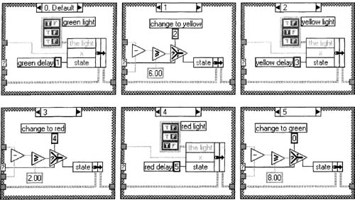
6.   Modify your cases as shown in Figure 6–15; then you should have a working VI.

      To get super-compact, we could have also combined the cases as such: 0-1, 2-3, 4-5, or 0-2-4, 1-3-5; but either of these formats would have been much more difficult to illustrate and understand.

      Compare Figure 6–11 to Figure 6–15, and you should be able to see an exact, one-to-one correspondence between states and cases.

7.   Run the VI, and you should see the traffic light on your front panel spend 6 seconds on green, 2 seconds on yellow, 8 seconds on red, then repeat the cycle until you stop the VI. If you’re still having trouble understanding how this works, you can run the VI with execution highlighting white watching the data in the block diagram, paying special attention to the input of the Case Structure’s selection terminal.

Figure 6–15
All six states of our state machine are implemented as cases of a Case Structure.

For simplicity, I’ve used integers to represent the states of a state machine. When designing a state machine in LabVIEW, you can use the Enum Constant from the Functions»Numeric palette so as to put the name of the state at the top of the Case Structure. The underlying data type will still be an integer ranging from 0 through whatever, but the Enum data type associates text with those numbers. When using an Enum Constant to control the state of a state machine in LabVIEW, it is wise to make it a typedef, as described in the previous section. To do this, strange as it may sound, you must start on the front panel and pick the Controls»Ring & Enum»Enum control, as shown in Figure 6–16.

After you drop this Enum control on any front panel, type in the following values, using the <Shift-Enter> trick when you want to add a new value:

0:   change to green

1:   green delay

2:   change to yellow

3:   yellow delay

Figure 6–16
Selecting the Enum control on the front panel.

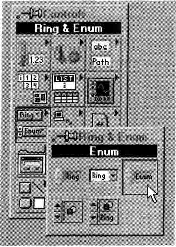
Figure 6–17
Six ring items on the front panel describe the states of our state machine.

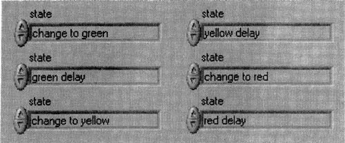
4:   change to red

5:   red delay

If you have added these six ring items properly, you should be able to see any one of these six values on the front panel object, as shown in Figure 6–17.

Figure 6–18
This block diagram is easier to understand and maintain than the one without the Enum.

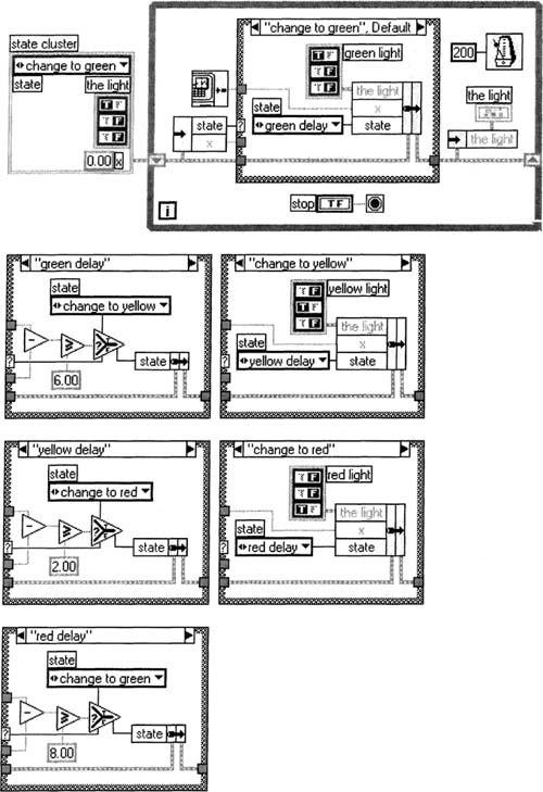
Save this Enum control as a strict typedef State Index.ctl, as described with the cluster in the previous section, then delete if from your front panel. At this point, since it’s been saved, you can use it on any front panel, or as we’re about to see, on any block diagram. A typedef has another advantage in state machines; if you want to add or remove a state later, the typedef will describe each state with text instead of with a number, making it easier to modify your states. Figure 6–18 shows how you should use your new Enum State Index .ctl to represent the state (it’s in the cluster constant on the left, too). Any custom control can be added to a block diagream as you would a subVI, with the Functions»Select a VI… menu item.

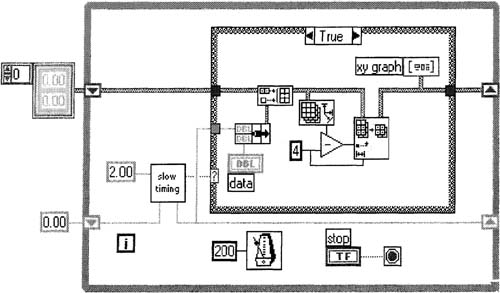
Technically, any time you have a Case Structure inside any loop, you have a state machine. Build the VI shown in Figure 6–19, using these tips:

Figure 6–19
A VI simulated simple, slow DAQ is shown.

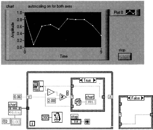
1.   Drop a Waveform Chart on the front panel. Pop up on the chart, turn autoscaling on for both axes, then create the free label as shown in Figure 6–19. Make sure the point style is set as shown. The plot seen will be created later.

2.   After you create the chart’s Property Node with the History Data property, you can pop up on this node and select Create»Constant to create the array of the proper data type.

3.   Save this VI as Simple Slow DAQ.vi.

Run this VI for about 20 seconds, so a plot like the one in Figure 6–19 is shown. Since these are random numbers, your plot will probably look different.

This block diagram illustrates how to implement very slow DAQ by executing a particular case of a Case Structure only at certain times—in this case, once every two seconds. If you wanted to collect once per minute, or once per hour, or at any rate slower than about once per second, this is a good technique. Notice how this timing differs from that in AI Single Point and Chart. vi, shown in Figure 3–37, and consider the difference in behavior when the computer’s processor delays for several times the desired sampling rate. In the earlier case, several samples might be taken in quick succession right after the processor’s delay, but for long tests, you will get a relatively constant number of samples over a longer period of time. I prefer this style.

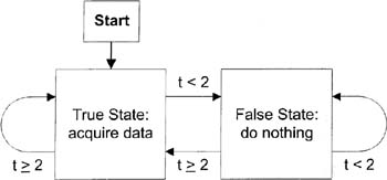
Figure 6–20 is a somewhat simplified interpretation of this VI as a state machine, where t is the time since the last execution of the True State:

Figure 6–20
A simple state machine is shown

Many times, you may want to use some DAQ input to control your program. If so, it sometimes helps to consider your VI as a state machine. Suppose you have a refrigerator or some other type of cooling mechanism, with a thermostat that turns the cooler on when the temperature drops below a certain value, then off when it rises above that same value. This is not a good implementation, because when the temperature is right at the critical point, any noise in the temperature-reading mechanism can cause the cooler to turn on and off very rapidly, thus reducing the life of the cooler—and irritating anybody within earshot.

For this reason, most temperature control mechanisms have hysteresis built in, which prevents rapid switching, as described in this paragraph. For temperature control, hysteresis defines a temperature range in which the cooler might be on or off depending on its previous value. For our imaginary refrigerator, let’s define this range as 35° to 40° F, and assume the ambient temperature is 70° F. If you turn the refrigerator on for the first time, the cooler will stay on until the temperature drops below 35°. Then, the cooler turns off until the temperature rises above 40°, at which point it turns on again. In other words, the refrigerator must remember whether the cooler was last on or off whenever the temperature is within the range 35° to 40° F. Figure 6–21 shows how it might work.

Figure 6–21
Typical temperature control with hysteresis is graphed.

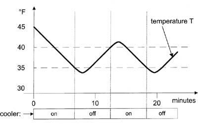
Figure 6–22 shows how a state machine could be designed to provide this type of control.

And finally, Figure 6–23 shows a VI that implements this functionality, where we are simulating the hardware with a front panel control (thermometer) and indicator (cooler). I’ve used a local variable in the block diagram so I can write to the cooler indicator from two separate cases—if this were a real DAQ control, we would likely have a digital output in the block diagram wherever we are writing to the cooler indicator. But the important point here is to notice how we first design a state machine’s functionality, then implement the states as cases in a Case Structure, just like we did earlier with the traffic light.

Figure 6–22
A state machine performing temperature control with hysteresis has these states.

6.1.3 Using Examples as Templates

In Chapter 3, we saw how to use an analog input example as a basis for our continuous acquisition VIs (your path may differ from mine):

C:Program FilesNational InstrumentsLV6examplesdaqanloin anlogin.llbCont Acq&Graph (buffered).vi

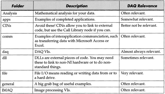
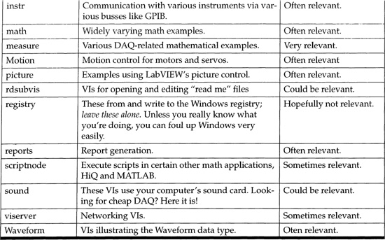
The most important point about using the examples is that you should immediately save them under a different name once you open them (see Appendix C). Failure to heed this warning can result in much time wasted. Figure 6–24 shows a quick overview of LabVIEW’s current examples folder. Table 6.1 provides information about the folders. See also Help»Examples….

Figure 6–23
A VI performing temperature control with hysteresis could be implemented as such.

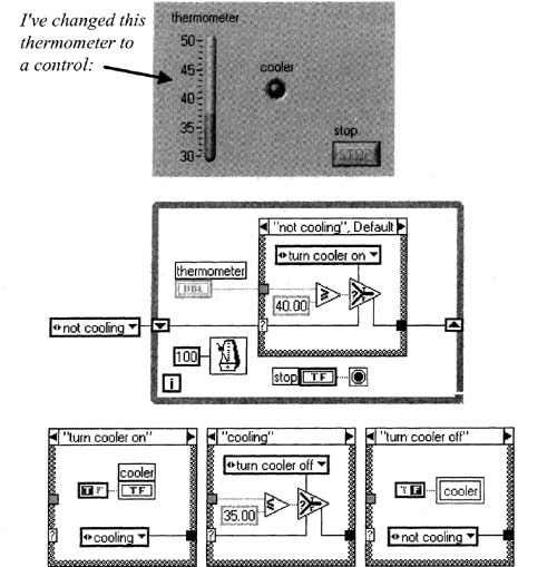
Figure 6–24
LabVIEW’s examples folder.

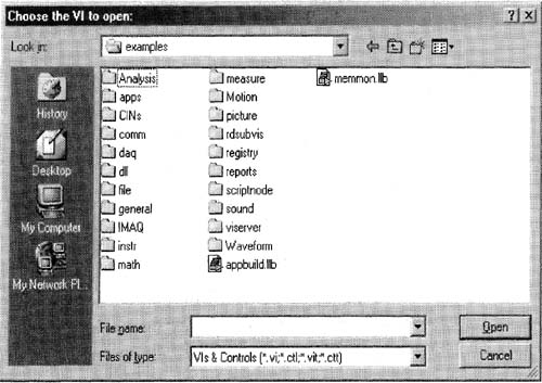
Table 6.1. Detailed descriptions of the items in LabVIEW’s examples folder

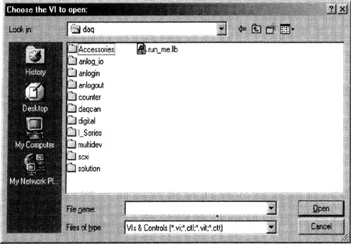
Let’s look into the daq folder now (see Figure 6–25 and Table 6.2). Take your time to browse around the examples—you don’t want to reinvent the wheel!

Table 6.2 Detailed descriptions of the items in LabVIEW’s examples/daq folder

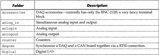
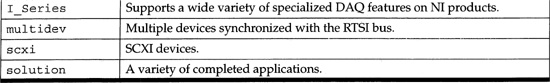
Figure 6–25
Here are some folders in LabVIEW’s examples/daq folder.

6.1.4 Handling Errors with Dialog Boxes

Handling dialog boxes white performing DAQ (or doing anything in LabVIEW) is inherently cumbersome. Why? Given a standard LabVIEW program with one main White Loop, user input and looping are suspended white the standard dialog boxes are showing from the One Button Dialog and Two Button Dialog functions.

Open Simple Slow DAQ. vi and save it as Dialog Boxes with DAQ 1. vi. Go to its block diagram, then build the following VI, using these tips:

1.   Streamline our timing code with the Select function, as shown in Figure 6–26, then select the portions shown.

Figure 6–26
Timing functions inside a block diagram are selected to make a generic timing subVI.

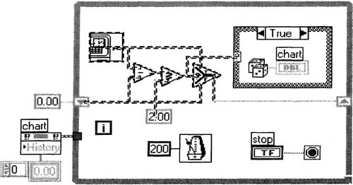
Figure 6–27
A generic timing subVI is created from the items selected in Figure 6–26.

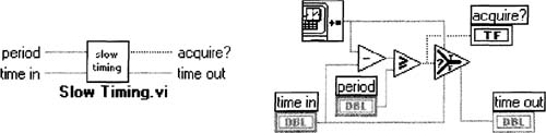
      Create a subVI from it, and save this subVI as Slow Timing. vi, creating the icon/connector and block diagram shown in Figure 6–27.

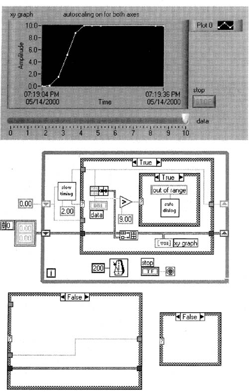
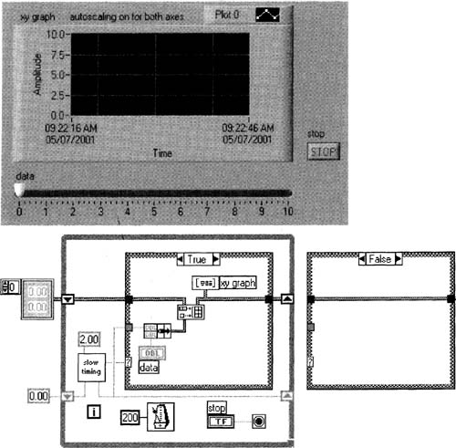
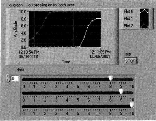
2.   On the front panel of Dialog Boxes with DAQ 1. vi, add the data Horizontal Pointer Slide control, as shown in Figure 6–28.

3.   Replace the chart with the XY Graph, and label it xy graph. Pop up on this graph, and using the X Scale»Formatting… menu item, change the Format: item to Time & Date. Ignore the data on the graph for now; we’ll create it soon enough. Each data point shown on the XY Graph is a cluster of two numbers, where the first number is the point’s x-coordinate (time), and the second number is the point’s y-coordinate (amplitude).

4.   Modify the block diagram of Dialog Boxes with DAQ l.vi as shown in Figure 6–28 by using the Bundle function, the Build Array function, and your previously created Safe Dialog.vi. The new constant wired to the lower left shift register is most easily created after everything else is wired by popping up on that shift register and selecting Create»Constant. The Build Array function automatically changes its upper element to an array type for you here.

5.   Save the VI again (as Dialog Boxes with DAQ l.vi) once you’ve successfully made these changes.

Set your data slide control to zero, run the VI, then raise data above 9.00 so you see the out of range safe dialog box pop up. Click its Continue button a couple of times, then leave the dialog box up for at least 10 seconds. Note that you cannot operate the data control when this dialog box is up. Finally, click Continue again, then stop the VI however you can.

The resulting graph might look like the one shown in Figure 6–28—see the gap between the data points? In this implementation, the dialog box interferes with the DAQ timing, thus causing the gap. We would like to continue acquiring data every two seconds, even when the dialog box is up. We would also like to able to operate front panel controls, like the data slide control, when the dialog box is up. Let’s fix these problems by building some custom VIs.

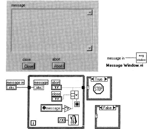
First, let’s solve the problem by using an even safer dialog box than the one we have; the one we have blocks all user input from our main screen whenever it pops up. Technically, we can no longer call this a dialog box, as a dialog box, by definition, blocks all user input from its parent window—so we’ll call it a message window. Build the VI shown in Figure 6–30 using these instructions:

1.   Notice that the message in terminal on the block diagram has no visible control on the front panel. To make this happen, create a message in string control on the front panel, then hide it to the left of the window by sizing the window and using the scroll bars.

2.   Create the global variable message as a string in your previously created Globals .vi.

3.   The Functions»Comparison»Empty String/Path? function tests for an empty string, and the Functions»Application Control»Stop function will stop all Vis.

Figure 6–28
This VI has a dialog box that halts DAQ when it shows.

4.   As this is a special VI used to pop up and display messages, go to File»VI Properties…, select the Window Appearance category, select the Custom radio button, then push the Customize… button to set the following screen, shown in Figure 6–29.

5.   Save it as Message Window, vi.

Figure 6–29
This Customize Window Appearance window lets you customize front panels.

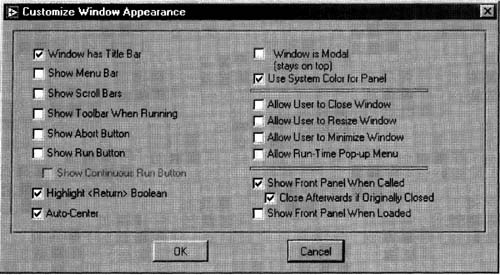
Figure 6–30 shows what Message Window. vi should look like.

Message Window. vi is designed for use as a subVI in a calling VI. Notice how the Show Front Panel When Called button is checked in the Customize Window Appearance window. Whenever you have Show Front Panel When Called checked, you should usually check Close Afterwards if Originally Closed checked as well. Since that Show Front Panel When Called property is set, be sure to have Message Window. vi closed before you run its calling VI.

Figure 6–30
This is one way to implement a dialog box that does not halt DAQ when it is showing.

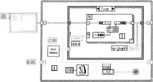
Save Dialog Boxes with DAQ l.vi as Dialog Boxes with DAQ. vi, then modify it as shown in Figure 6–31 (I made it as simple as I could, honest), using these tips:

1.   Two local variables are created from the stop button. Set the stop button’s mechanical action to a non-latching value; local variables are not allowed with latching buttons. The front panel should look the same as it did, however, so we won’t show it again here.

2.   Create the global variable String Control message in Globals. vi, and use it as shown on the block diagram.

3.   Be patient; it takes a lot of work to handle this seemingly simple situation.

Figure 6–31
This VI illustrates a dialog box subVI that does not interfere with main VI’s execution

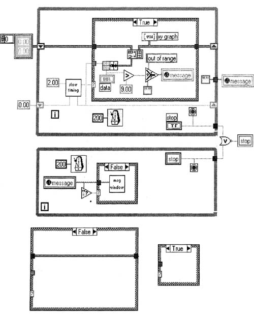
The main trick here is having two White Loops running simultaneously. If we display a standard dialog box window from our upper loop, it stops and therefore DAQ stops—so we need another loop to display a message box. The upper loop acquires the data, and the lower loop displays the message box. When the upper loop discovers a data value greater than 9, it sets the global variable message to out of range. When the lower loop detects anything but an empty string, it calls Message Window. vi, which pops up and displays the message. Notice that the lower loop stops whenever the message window is showing, so Message Window, vi must monitor the message global internally so it can automatically close itself whenever there is no message. We set the message global to an empty string when the upper loop stops so the message window closes itself if it’s showing.

The stop button uses its two local variables to stop both loops at once, and then to reset itself to its original state.

6.1.5 Monitoring Bus-Based Ports

Don’t bother building the VIs in this section, unless you have a null modem cable, two computers with LabVIEW and serial ports, and the desire to actually do bus-based programming.

Many times, you might have external equipment that communicates via a bus, such as the RS-232 port. Although this might not fall under the strict definition of DAQ, it’s close enough for me, and it’s often used with DAQ, so this section discusses the key issues. I will be using the RS-232 port, as most computers have these, but the basic concepts herein apply to all bidirectional ports.

Suppose your computer will be connected to an RS-232 gadget that can read and write data.

Some RS-232 devices only write data, sending out a constant stream of information, but we won’t discuss that in this book, as it’s really a subset of the read/write scenario.

Suppose you want to acquire a piece of data from this read/write gadget; you will usually need to send the gadget a special “request” code. This code will vary per gadget. The gadget then responds with the data, which may be in binary or ASCII format. You need to read the gadget’s manual to figure out how to decode this data.

Before any communication at all will work, you may need to set some low-level hardware parameters relevant to your particular port. For an RS-232 port, these parameters are usually baud rate, number of data bits, number of stop bits, and parity. Hardware control can also be tweaked, but this is usually not needed. You must make sure these parameters match your serial gadget’s settings, or you will get garbled data, if any.

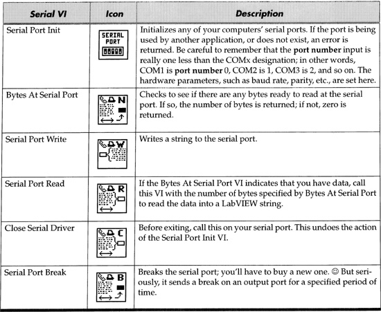
LabVIEW 6i introduced a new set of serial I/O VIs in the Functions»Instrument I/O»Serial palette, with the word VISA attached. I prefer the older-style Vis, found in the Functions»Instrument I/O»I/O Compatibility»Serial Compatibility palette, because they are currently more reliable. Figure 6–32 shows a comparison of the two palettes, and Table 6.3 describes the serial Vis. The left palette does have the advantage of more elegant error checking, by using the error cluster, and I would recommend using them for this reason if you can get them to work reliably.

Figure 6–32
The Serial palette and the Serial Compatibility palette.

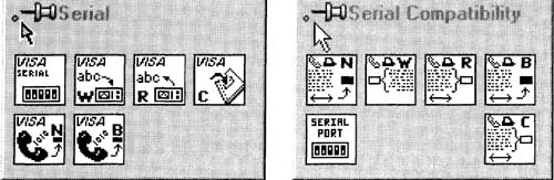
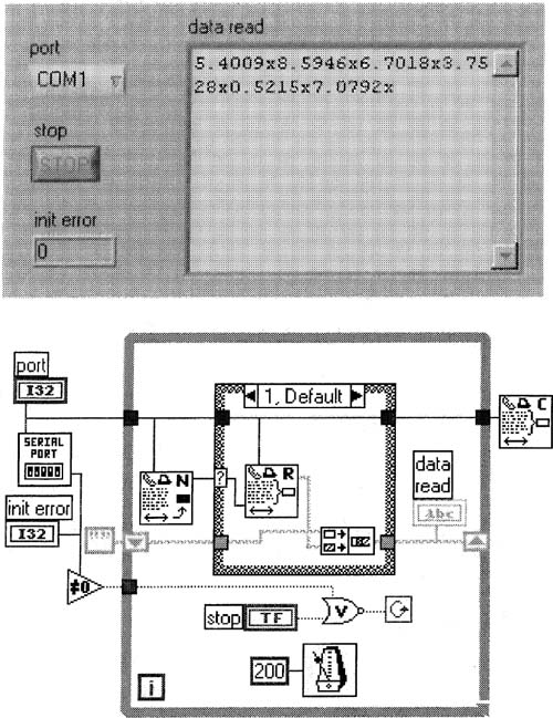
Figure 6–33 shows a very simple VI that monitors the serial port for data, and reads it into an ever-growing string.

In a real system, you would want to empty the string in the Shift Register after you’ve read valid data, to keep that string from getting too large. And to be more robust, you would want to check for errors on all the serial VI functions. I have foregone this error checking for the sake of simplicity here, except for init error, which in my experience is the only error that ever occurs (when a port is not valid for whatever reason). To implement more professional error checking, use the error cluster as in the VISA versions of serial VIs, or as in file I/O Vis, by wrapping a VI around each of these serial VIs.

The data in the data read indicator shows what came through the serial port. I specifically set my system up so we could read ASCII bytes, but your serial gadget may give you non-ASCII bytes. Notice the very important Concatenate Strings function. If you read the serial port in mid-message, you may only get the first few bytes of a multibyte string; the shift register saves this and tacks additional bytes, if any, onto the end of your first few bytes on the next iteration of the loop.

Table 6.3. Detailed descriptions of the items in the Serial Compatibility palette

A serial gadget could have written this data. To verify this VI’s operation for this book, I built a different VI running on a different computer, connected with a null modem cable, which wrote the data you see—I rigged the data so that every character is a readable ASCII character. A null modem cable allows two computers to connect directly to one another—on a basic 9-pin null modem cable, lines 2 and 3 are crossed, and line 5 is connected directly. The other six lines may remain unconnected unless you want hardware handshaking. Figure 6–34 shows the VI running on a second computer that wrote the data in the previous figure via null modem cable.

Figure 6–33
A simple serial port monitor.

Like the previous VI, you would want to check for errors on all the serial VI functions. This VI writes the bytes in data to write to the specified serial port whenever the write button is pushed. The write button must have a latching mechanical action.

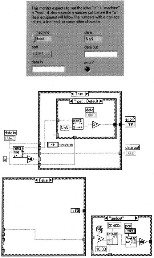
I will now put together a VI that simulates a typical serial gadget. The VI will also double as a VI running on a host computer monitoring that serial gadget. I have here in my office two computers connected via null modem cable. Both computers have LabVIEW and a COM1 serial port. One of my computers, I will call the “gadget,” as it will be simulating a serial gadget, and the other, I will call the “host” as it will simulate a computer with a real serial gadget. The gadget will transmit a random number in the range 0 to 10 to the host upon request. The magic letter here is “x” for both computers. The gadget will send an x when it is finished transmitting its random number, so that the host will know when to interpret its received bytes as a complete number. For example, if the gadget wanted to transmit a 1.9, it would really transmit 1.9x. That way, if the host sees just a 1, it knows there’s more coming, and it stores the 1 in its shift register. It then gets a .9x, or at least some of it, on the next iteration of the loop. The computer requests a random number from the gadget by sending it an x. Sound complicated? Well, this is basically the way most bus-based instruments work, serial or not—they request data from an instrument by sending a command, then wait for the data, and be prepared to receive it on the next bus read or reads.Figure 6–35 shows Serial Monitor. vi, which runs on both the gadget computer and the host computer.

This block diagram is sloppy because of how we’re checking the errors—in fact, we might not even know exactly where the error came from! But it is more concise than doing it the correct way, which would be to wrap each serial VI in another VI which uses the error cluster, then daisy-chain the serial VIs together. Or, use the newer version of serial VIs that have already done this for you! Here, however, we’ll save much time by checking the errors in this clumsy fashion. Here is a list of the important points to recognize:

Figure 6–34
A simple serial port writer.

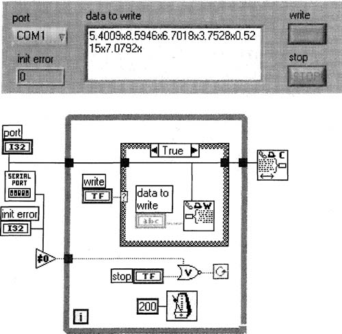
Figure 6–35
This VI works, but the error checking is very awkward and takes up much space. See your other options below.

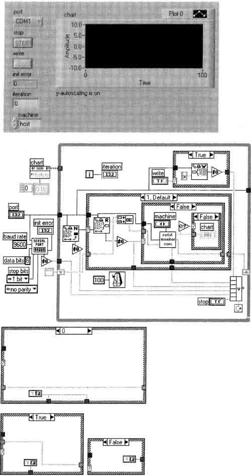
1.   This VI will run on both computers, and it continuously monitors the serial ports for data on both computers. The gadget computer is looking for a lone “x”, and the host computer is looking for a number followed by “x”, like “2.7183x”. When data is found, it is sent to Serial Monitor Core. vi, which is customized to run differently on the two computers.

2.   Like the simpler serial reading VI shown previously, we should use the Concatenate Strings function with a shift register to make sure that we piece together data in case it’s received on different iterations of the White Loop.

3.   The wire entering the largest Case Structure’s selection terminal indicates how many bytes of data are waiting at the serial port to be read. By making case 1 the default case, this technique will read the data whenever there are more than zero bytes available (not just one byte).

4.   Serial Monitor Core. vi returns NaN (not a number) whenever it gets numeric data that is not followed by an x. The little triangle to the right of Serial Monitor Core. vi is the Not A Number/Path/Refnum? function , and it uses the smallest Case Structure to write data to the front panel chart only when the data is valid (followed by an x).

5.   The Case Structure with Serial Write .vi writes an x whenever the write button is pushed. The write button must have latching mechanical action.

6.   The logic connected to the White Loop’s conditional terminal stops the main loop whenever an error occurs or whenever the stop button is pushed.

7.   On the front panel, I made the port ring a typedef and saved it to disk, so I can use this as the COM port control for all my serial Vis. Its values are COM1, COM2, COM3, and COM4, which conveniently correspond to the values 0,1, 2, and 3, respectively. You can go higher than COM4 if need be by simply adding more items to the typedef.

Let’s go down one more level and look at the guts of Serial Monitor Core. vi, as there are some useful concepts there. See Figure 6–36. Here are the key points of this subVI:

1.   The default value of data is NaN (not a number), so that whenever something other than a number is written to it, this VI outputs a NaN through data.

2.   The powerful Match Pattern function searches the incoming string for the letter x. If no x is found, the False case of the main Case Structure is executed, which simply passes any data in the shift register of Serial Monitor. vi back to the shift register, unchanged.

3.   Data may arrive in incomplete chunks. If an x is found by the Match Pattern function and data is found after the x, that data is saved for the next iteration of the main White Loop, because it’s part of the next number to be sent. This is a key point in any bus-based LabVIEW acquisition—don’t throw away any data! That’s the purpose of the wire going into data out in the True case in Figure 6–36; it will pass this incomplete data to the next iteration of the White Loop. In that same case, the wire passing through the inner Case Structure’s host case contains all data before the x, which should be a complete floating-point number in string form.

4.   The outer Case Structure is executed whenever an x is found on a serial port, regardless of the computer. If we’re on the gadget computer, the computer ring will be set to gadget and a random floating-point number with four digits of precision will be written to the serial port. Remember the data

5.4009x8.5946x6.7018x3.7528x0.5215x7.0792x,

      in our simple serial-read VI shown in Figure 6–35? This was the result of six such numbers being read in succession. The other case of the inner Case Structure executes whenever an x is seen on the monitoring computer, in which case the data before the x is interpreted as a floating-point number, and sent to the data indicator to be charted by our calling VI, Serial Monitor. vi.

In real life, you will probably never see the letter x used as a delimiter. I only used it here because it’s easy to see. More often, the delimiter is a carriage return, line feed, comma, tab, or space.

Figure 6–36
Our serial VI reads and writes formatted data.

Some serial devices output a constant stream of data without being asked, not unlike my last girlfriend. If you get such a device (a serial device), take care to not misinterpret incomplete data when you begin receiving. For example, let’s pretend you started reading the stream 5.4009x8.5946x6.7018x midway into the first number, so you read 009x8.5946x6.7018x. You have no way of knowing whether that first 009 is valid, so ignore any data until you get past your first delimiter. In this case, the first number you should take seriously is 8.5946.

Before leaving this section on busses and ports, you should learn one more trick about what to do when you are monitoring multiple ports. Suppose you have eight devices connected to eight serial ports on your computer. Suppose also that each device takes about 400 ms to respond to a data request. If you request data from one device and wait for it to respond before requesting from the next, you will be waiting 3200 ms, or 3.2 seconds, to read data from all eight devices; this will introduce an annoying delay to the responsiveness of your program! Instead, you should send requests to all eight serial devices, then wait for each one to respond in a loop. Remember the string we’ve been keeping in a shift register for serial monitoring Vis? We will now need an array of eight strings in a shift register, one per device, as each device will be collecting data independently in its own string. This sort of LabVIEW program will grow complex, and you’ll likely need to send this array of strings to subVIs, so don’t forget the typedef trick mentioned in the first section of this chapter.

6.1.6 Multiplot XY Graphs

Suppose you want to acquire data for a long period of time (anywhere from a few seconds to a few years) and show the data on a graph with timing information on the x-axis. Usually, you’ll want to do this with a very slow sampling rate, 1 Hz or slower. If this is what you want, this section is for you, because XY Graphs are good at showing such timing on their x axes.

Open Dialog Boxes with DAQ 1. vi from earlier in this chapter and save it as Multiplot XY Graph. vi. Modify this VI as shown in Figure 6–37, then save it again.

This VI simulates analog input of one channel of data, where the data is controlled by you from the front panel slide control data. Suppose you want to expand the above VI to accommodate multiple channels. I’m tempted to just gloss over this topic, and say “read the fine manual” concerning multi-plot XY Graphs, and expand your data types as such. But there’s some trickery involved, so we should explicitly work through a multiplot example.

If you want to find out exactly what the multiplot data types are for the XY Graph, you’ll need to dig through LabVIEW’s Help documentation to find it. I finally found this description in LabVIEW’s User Manual:

Figure 6–37
An XY Graph will be used with simulated data.

The multiplot XY graph accepts an array of plots, where a plot is a cluster that contains an x array and a y array. The multiplot XY graph also accepts an array of clusters of plots, where a plot is an array of points. A point is a cluster that contains an x value and a y value.

Refer to theXYGraph VI in the examplesgeneralgraphgengraph.llb for an example of multiplot XY graph data types.

Figure 6–38
XY Graph data types.

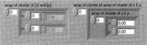
The two data types described above would look like Figure 6–38 on the front panel (the example listed shows you the same data types on the block diagram).

I’ve always preferred the second of these two data types, as the first form allows differently sized X and Y arrays, which is useless to an XY Graph. The second data type neatly bundles the X and Y coordinates of each data point.

1.   Delete the appropriate objects on the block diagram of Multi-plot XY Graph. vi, as in Figure 6–39.

2.   On the front panel, replace the data slide control with an array of three such slide controls having values of roughly 0,1, and 2. Make this array the default value, or you’ll have an empty array next time the VI is opened. White you’re on the front panel, change the graph’s legend to have the point styles shown in Figure 6–40.

Figure 6–39
A VI using an XY graph is being built.

      If you’ve forgotten some of Chapter 1, which is quite understandable, you need to use the Positioning tool to grow the data array to show three slide controls, then switch to the Operating tool to change the data to approximately 0,1, and 2.

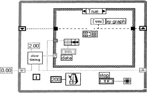
3.   Build the block diagram shown in Figure 6–41, saving the complex-looking constant of arrays and clusters at the far left

      until last, at which point you can pop up on the left shift register and select Create»Constant. The functions inside the For Loop are the Bundle (two of them), Unbundle, and Build Array functions.

This VI appears to be set up to plot data every two seconds. Run this VI, and notice that it does not plot data at all.

Figure 6–40
A front panel using slide controls for DAQ simulation is shown.

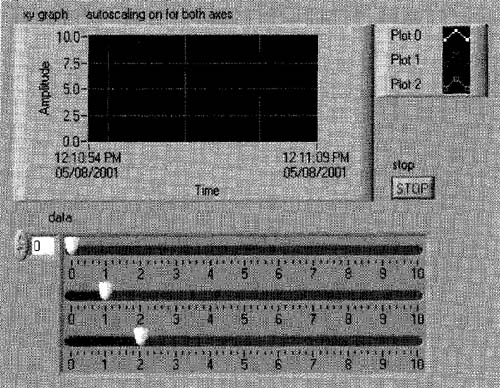
Figure 6–41
This VI might make you think it will plot data, but mysteriously, it does not.

What’s going on here? Who said LabVIEW was simple? Don’t look at me! if you understand why the data is not being plotted right away, maybe you don’t need this book.

Let’s analyze this block diagram. Every two seconds, the True case of the Case Structure executes. The For Loop should iterate three times, since we created an array of three elements on the front panel. Each iteration of the For Loop appends another data point onto the corresponding array of data points for each of our three plots.

So why won’t the data plot? The data in the shift register appears to be an array of clusters of an array of clusters of X and Y data points. But in reality, the constant initializing the shift register is an empty array. This means the For Loop will execute zero times, not three, because its smallest array input has size zero! You can verify this by running the program with execution highlighting on and watching the block diagram. How do you correct this? You could modify that complex-looking constant to be an array of three clusters of empty arrays, but that’s awkward and leaves a hard-to-read block diagram. I prefer the method shown in Figure 6–42, in which you drag the cluster out of the complex-looking array constant and use the Initialize Array function.

I’ve run this VI, slowly changing each slide control, to produce the graph in Figure 6–43.

Figure 6–42
The VI from Figure 6–41 is cured.

Figure 6–43
Our XY Graph VI, plotting simulated DAQ data, finally works! The plots correspond to how the slide controls were moved by the user.

6.1.7 Limiting Graph Data Size

Regardless of your scan rate, you might get to the point where the graph data becomes too large, and you only want to see the last section of the graph. A chart will do this automatically for you if you set its history length, but you’ll need to programmatically control the length of any sort of non-chart.

Usually, you’ll want to track the last few hundred or few thousand data scans on a graph. To keep things really simple, suppose you wanted to only show the last four scans of data, and you’re acquiring one point of data per iteration of a White Loop; see Table 6.4.

Table 6.4. Eight iterations of a loop are shown in which only the last four elements of an array are retained.

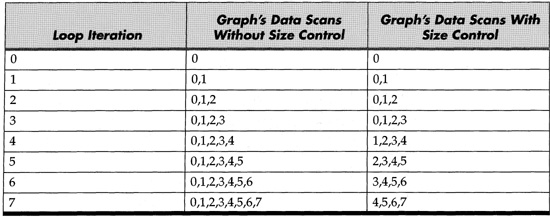
Let’s add this functionality to our Dialog Boxes with DAQ l.vi;save this VI now as Last Four AI Points. vi, and we’ll modify it so we are only looking at the last four simulated scans. In the real world, you’ll more likely want to see a few hundred or a few thousand scans, but four will illustrate the technique here.

Change the block diagram as shown in Figure 6–44 by adding the Array Size, Subtract, and Array Subset functions.

If you now run Last Four AI Points .vi, you can see how the Array Subset function is always taking the last four points of data stored in the shift register. If you’re really sharp, you will have noticed that when the first point is added to the shift register, the Array Subset function gets a -3 in its Array Index input and a 4 in its Array Length input. Luckily, the Array Subset function is smart enough to not crash your computer, which might have happened had you been programming in a text-based language! Instead, the clever Array Subset function internally changes the -3 to a 0, and the 4 to a 1, thus doing the right thing. All LabVIEW functions that manipulate arrays are similarly clever—yet another reason to use LabVIEW!

Figure 6–44
This VI looks at only the last four data samples by exploiting the Array Subset function.

6.2 ANALOG WAVEFORM ANALYSIS

Suppose you are running a test and must analyze some analog data. If acceptable, collect all of your data first in an array or file, then once the test is complete, analyze your data as a LabVIEW array. But if you need to analyze the data white the test is occurring, it can be tricky. In this section, we will demonstrate analysis occurring while data is being acquired continuously.

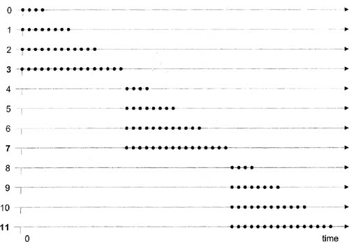
Two different buffering methods will be presented in this section. These buffers are not the hidden buffers that NI-DAQ uses during continuous acquisition; we will explicitly create these buffers with LabVIEW arrays. Suppose you are continuously acquiring analog data at a constant rate, with four scans per iteration of a White Loop. Figures 6–45 and 6–46 illustrate two buffering mechanisms you could use. These diagrams illustrate how data is buffered per iteration of the acquisition loop. The bold numbers towards the left indicate the iterations in which an analysis takes place—whenever our 16-sample buffer is filled with new data. For this example, let’s pretend we’re taking 20 samples per second (20 Hz), but acquiring only four data points at a time, although real applications often involve much higher data rates and correspondingly many more data points sampled at a time.

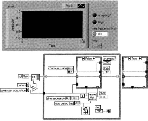
Open Simulate AI Waveform. vi which you should have built in Section 4.1.1, save it as Continuous AI Analysis. vi, and modify it as in Figure 6–47, using these tips:

1.   Give the sgl Numeric Constant an SGL data type via its Representation pop-up menu.

2.   The Initialize Array function is used.

Figure 6–45
Buffering during continuous analog acquisition is illustrated where data can be analyzed every iteration once the buffer is filled

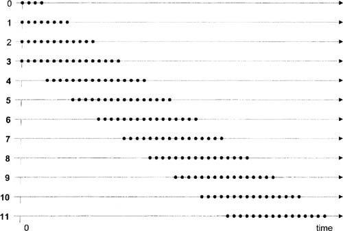
Figure 6–46
Buffering during continuous analog acquisition is illustrated so that data can be analyzed less frequently than in Figure 6–45.

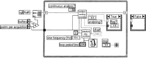
Create a subVI by selecting the Case Structure in Figure 6–47 then using the Edit»Create SubVI menu item. Save this new subVI as Analyze Analog Waveform.vi. The block diagram of Continuous AI Analysis. vi should like Figure 6–48.

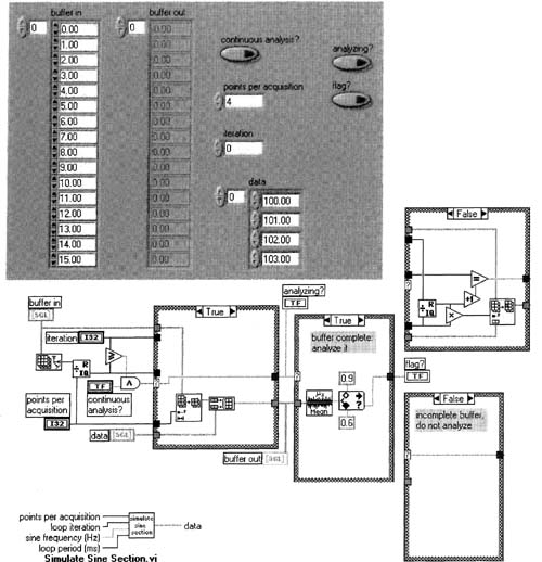
Modify Analyze Analog Waveform. vi as shown in Figure 6–49 using these tips:

1.   Make sure the iteration terminal is the one connected to its calling VI’s White Loop’s iteration terminal (shown in Figure 6–48).

2.   In the short fat Case Structure, the Replace Array Subset function and the Build Array function are in the Functions»Array & Cluster palette. You will need to pop up on the Build Array function and check its Concatenate Inputs menu item—otherwise it will produce a 2D array rather than the ID array we want.

Figure 6–47
Continuous AI Analysis.vi is prepped for continuous analog acquisition.

3.   In the tall skinny Case Structure, the In Range and Coerce function is in the Functions»Comparison palette. Mean. vi is found in the Functions»Mathematics»Probability and Statistics palette.

4.   If you replace the numeric elements of buffer in and buffer out with those shown (from the Controls»Classic Controls»Numeric palette), your array elements will line up with one another.

Enter the front panel data shown. Repeat the following procedure at least a dozen times or until you can see how this implements the buffering scheme shown in Figure 6–46.

Figure 6–48
Continuous AI Analysis. vi is prepped further for continuous analog acquisition.

1.   Run the VI with the <Ctrl-R> key.

2.   Look at where the data appears in the buffer out array.

3.   Click the up arrow on the iteration numeric control so its data is incremented.

Set the iteration numeric control back to zero, set the continuous analysis? control to True on the front panel, then repeat the recent three-step procedure at least a dozen times or until you can see how this implements the buffering scheme shown in Figure 6–45.

Let’s explain what’s going on here with respect to the block diagram. As you can see from Figures 6–45 and 6–46, the first four iterations of the two buffering mechanisms are identical, in which case the False case of the short fat Case Structure of Figure 6–49 is executed. The Replace Array Subset function in that False case clearly replaces a subset of the array. After the fourth iteration, the two buffering mechanisms differ. The mechanism of Figure 6–46 will continue to use the False case. The mechanism in Figure 6–45 will use the True case of the Case Structure, which simply strips off the first four points of the buffer and appends the new four points, exactly as Figure 6–45 suggests.

Figure 6–49
Analyze Analog Waveform. vi is shown.

Run Continuous AI Analysis.vi with its sine frequency (Hz) numeric control set to 0.1. Try other frequencies, never more than about 4 Hz, and experiment with the continuous analysis? constant on the block diagram of Continuous AI Analysis. vi. Once you know that the flag? indicator should be true whenever the last buffer analyzed has an average in the range of 0.6 to 0.9, and if you keep in mind Figures 6–45 and 6-46, everything should make sense. If your frequency is too high, the flag? indicator will not light.

Notice that the continuous analog input acquisition examples that ship in LabVIEW’s examples folder (mentioned in Chapter 2) output 2D arrays of data, whereas our example here was working with a ID array. In general, our VIs in this section could be modified to work with 2D data by adding a dimension to the ID arrays and dragging For Loops around the functions connected to your new 2D wires. You will run into a few other array-related issues depending on how your VIs are built, but that’s the basic approach for converting from ID math to 2D math.

6.3 FILE I/O FOR DAQ

This section will discuss a few diverse file I/O topics pertinent to DAQ.

6.3.1 Binary data files

In order to understand this section, you must not only understand bits and bytes, but you must understand LabVIEW data types and the difference between binary and ASCII data. These topics are covered in Appendix A and Chapter 1.

Let’s use one of the VIs from Chapter 3 that saved ASCII data, and we’ll modify it to save binary data. Open AI Single Points and Chart. vi along with our recently created Multiplot XY Graph, vi. Since we’re not using any real DAQ devices in this chapter, save AI Single Points and Chart.vi as AI Single Points and Chart (sim) .vi. Modify your new VI as in Figure 6–50, using these tips:

1.   Copy the data array of slide controls from the front panel of Multiplot XY Graph, vi to the front panel of your new VI. Empty this array with its Data Operations»Empty Array pop-up menu item, then make it a two element array having values 0 and 1. Make this the array’s default value. You may close Multiplot XY Graph. vi now, as we only wanted it for its slide controls.

2.   Replace all the real DAQ stuff on the block diagram with the data terminal from your array of two slide controls; we’re simulating all data in this chapter.

3.   Enter a valid path to a file we’ll create, called ascii4. txt in the file path control. Your path will likely be different from mine, of course.

Run the VI for about 10 seconds, changing the slide controls as you wish, so you get some changing data on your chart. For example, I get the data shown in Figure 6–51.

Now, open your Read and Display CSV Data. vi and copy the path to your ascii4 . txt file into its file path control. Run the VI, and you should see the same data you created. This data was written to disk in ASCII format.

We will now write similar data to disk in binary format. Save AI Single Points and Chart (sim) .vi as AI Binary Save (sim) .vi. From its block diagram, open Write ID Ascii Data. vi, and save it as Write ID Binary Data. vi with the File»Save As… menu item, which effectively replaces itself in the block diagram of AI Binary Save (sim) .vi. This will be more apparent when you update these Vis’ icons to reflect their new file names. Modify your new Write ID Binary Data, vi as follows, using these tips:

1.   On the front panel, remove the data string control.

2.   That new oddly shaped function (see Figure 6–52) is the Type Cast function, which converts binary data to string data. It is found in the Functions»Advanced»Data Manipulation palette. The file I/O VIs accept string data as their default data type at the lowest level. There are specialized VIs that could have saved this floating-point data without explicitly using Type Cast function, but this is a more powerful technique in that it can be easily modified to many data types.

3.   Make the icon look like this:

4.   Your block diagram for AI Binary Save (sim) .vi should look much like Figure 6–53, if you’ve followed the instructions carefully.

5.   On the front panel of AI Binary Save (sim). vi, change your path so that you’re writing to ascii4.bin rather than to ascii4. txt, making it the default value as well.

Figure 6–50
This VI writes simulated DAQ data to disk in ASCll format.

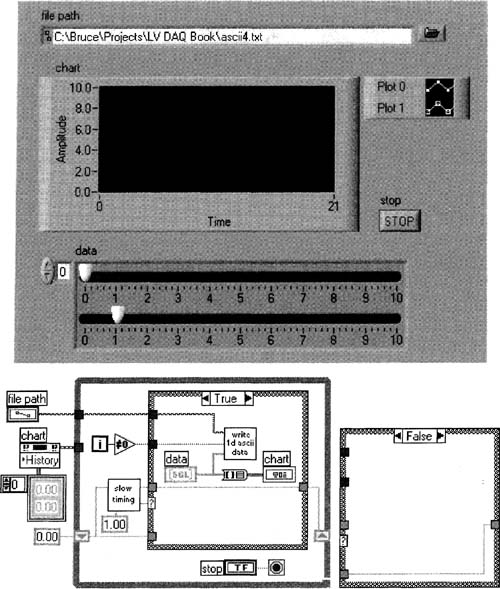
Figure 6–51
These plots represent data corresponding to the movements of the slide controls in Figure 6–50.

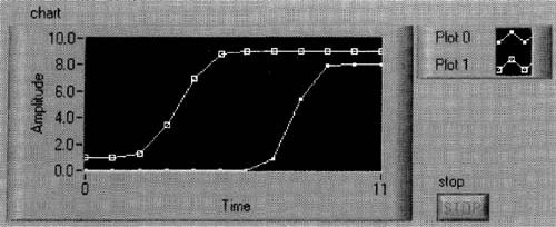
Figure 6–52
This snippet of code uses the Type Cast function to convert data to binary format then write it to a file.

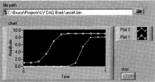
6.   Run your VI and change your data slide controls white it’s running, so you see some data looking something like the plots in Figure 6–54.

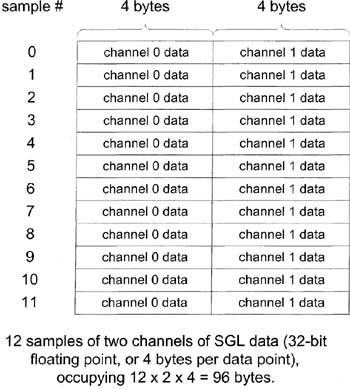
First, understand what your data “looks" like on disk if you happened to get exactly 12 samples (at two data points per sample). See Figure 6–55.

Figure 6–53
This block diagram is a modification of an earlier VI so that is saves data in binary format rather than ASCII.

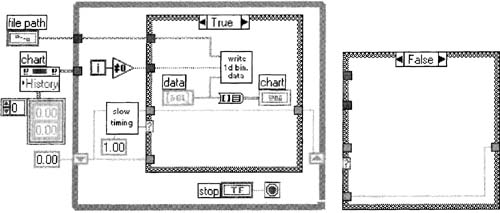
Figure 6–54
This familiar front panel is used for saving binary data, not ASCII as before.

Here’s how to read that data. Open your Read and Display CSV Data. vi, if it’s not already open, and save it as Read and Display 2D SGL Data.vi. Now, make it earn its name by modifying it as follows (and saving it afterwards):

1.   Copy your ascii4. bin path’s text to the file path control of this VI, making it the default value.

Figure 6–55
Binary data is illustrated.

2.   Given our very raw form of binary data, we must tell our data-reading VI how many columns, or channels, of data we have. Add a channels numeric Digital Control, and give it a value of 2, since we just acquired two channels of data. See Figure 6–56.

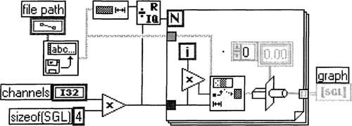
3.   Now, let’s fix the block diagram so it is expecting a simple 2D array of SGL (single precision, or 32-bit, floating-point data). See Figure 6–57.

This VI takes a string of bytes and breaks it into substrings such that the length of each substring corresponds to each scan. The Type Cast function, which just recently changed binary data to string data, now does exactly the opposite—it changes string data to binary, because we wired its center terminal. You might ask, why didn’t we just skip the For Loop altogether and wire a 2D array of SGL data? Answer: The Type Cast function can only deal with very simple types of data. For more complex types of data, you could use the functions described in the next paragraph.

Figure 6–56
This front panel will display our recently created binary data.

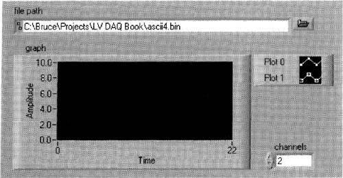
Figure 6–57
This block diagram is used to display our recently created binary data.

Suppose that you saved all your DAQ data in memory, rather than writing it to disk one piece at a time. There’s a really simple way to write any data, even very complex data, to disk in LabVIEW—the Flatten To String function. Like the Type Cast function, it is in the Functions»Advanced»Data Manipulation palette. The binary data from the Flatten To String function will have some header information at the beginning, which helps decode the data format later, but other than that, this data looks similar to data created by the Type Cast function. To display the data, use the Unflatten To String function, passing the exact same data type to one of its inputs (this input ignores the data, but just looks at the data type), and you have your complex data.

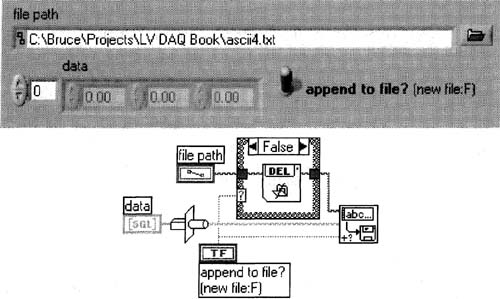
6.3.2 Automatic Data File Organization by Date

You might not agree with my strategy in this section when you first hear it (most people don’t at first), but I’ve been using this trick for many years now, and this turns out to be a very effective strategy. Until Windows 95 came out, we didn’t have the luxury of using long file names and folder names on the PC; but now we do, so let’s use them!

The VI in Figure 6–58 simply creates a new path for your test data, based upon the time and date.

Here are its advantages:

1.   Unless you’re creating a file more than once within a second, this VI automatically creates unique file names for you. If there’s a chance you’ll write more than once within one second, you may want to append an extra number, such as an “iteration” number, to the name.

2.   If you sort your file names alphabetically, they’ll also be sorted chronologically.

3.   The file subname control allows for data-dependent customization.

4.   You can categorize according to other criteria, such as your project’s name, by using the base folder.

I have yet to see any legitimate disadvantages to using this scheme.

6.3.3 When to Flush

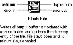
When you’re saving data to disk, and using the standard file I/O functions, the data may not be physically written to the disk until you flush, or close, the file. If your application continuously saves data to disk, your operating system sneakily buffers this data in memory, without telling you, until it decides to physically write to disk. This can result in noticeable delays if the buffer happens to be too large. To get around this, you can use LabVIEW’s Flush File function, which physically writes any and all file data from the sneaky buffer to the disk as illustrated in Figure 6–59.

Figure 6–58
This VI creates a path that contains the time and date. For repeated testing, this is quite useful for organizing data.

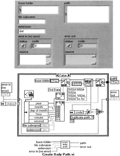
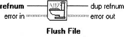
Figure 6–59
LabVIEW’s Flush File function.

The LabVIEW team immediately canned my idea for the Flush File function’s icon, shown in Figure 6–60, when I worked at NI.

Figure 6–60
Not LabVIEW’s Flush File function, just my quickly-rejected idea.

Some high-level file I/O functions open a file, write it, then close it, in which case flushing is not relevant, as file data is automatically flushed whenever a file is closed.

6.3.4 Databases

NI offers a SQL Toolkit (Structured Query Language; that acronym is pronounced sequel), which allows direct communication with most databases, such as Microsoft Access. Copying directly from NI’s Help window, here’s a summary of the SQL Toolkit’s features:

▪   Direct interaction with a local or remote database

▪   Connection to most popular databases

▪   High-level, easy-to-use VIs for common database operations

▪   Complete SQL operation

▪   Low-level VIs for direct access on columns, records, and tables

If timing or speed is not an issue, skip this paragraph. Be warned that SQL functions can take much more time to execute than LabVIEW’s file I/O functions. Also, it’s rather easy to use the SQL Toolkit in an inefficient manner, so make sure you are familiar with SQL speed issues independently from LabVIEW. Another way to speed up database acquisition is to write your data to your own custom database white acquiring, then convert it to your target database format later, when timing is not critical.

If your database does not support SQL, look in the Functions»Communication palette to see if another means of communication is applicable.

6.4 AVERAGING

Averaging is a technique for reducing noise in signals. You should try to reduce the noise via hardware techniques, as described in Chapter 1. There are software filters other than averaging built into LabVIEW, which you may find more useful, particularly if frequency response is an issue. For a full technical description on the effects of averaging, see NT’s Application Note 152, Reducing the Effects of Noise in a Data Acquisition System by Averaging. The brightest analog engineer I know, who also happens to have the shortest email address I’ve ever seen (coincidence?), wrote this app note; here’s his summary of averaging at the end of said app note, where i.i.d. means “independent and identically distributed."

Underlying the application of averaging or filtering is a trade-off between the degree of certainty achieved and the number of samples that must be taken (and the time it takes to obtain them). When samples are independent and identically distributed, averaging a collection of samples reduces measurement uncertainty by a predictable amount. If o is the amount of rms noise in a set of n i.i.d. samples, the rms noise of the average taken over the samples is

Suppose the your rms (root mean square) noise on a 0 to 10 volt signal is 0.1 volts. By taking the average of 100 “independent and identically distributed” samples, which is easy to do with the DAQ Vis, you will have reduced your noise by a factor of 10, so your rms noise is effectively 0.01 volts.

Suppose you have the following data samples:

1, 2, 3, 4, 5, 6, 7, 8, 9, 10, 11, 12

Next, suppose you are taking the average of four points. To get “independent” data, you must average “1, 2, 3, 4” “5, 6, 7, 8” then “9, 10, 11, 12” as opposed to “1, 2, 3, 4” “2, 3, 4, 5” then “3, 4, 5, 6". In other words, you should not use any of the same data from one averaged sample to the next, as this is not independent information.

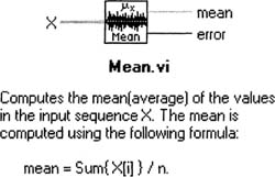
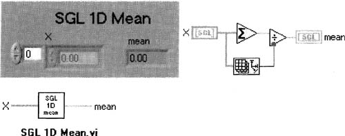
LabVIEW ships with an averaging VI called Mean. vi (mean means average), to be found in the Functions»Mathematics»Probability and Statistics palette (see Figure 6–61).

Figure 6–61
LabVIEW’s Mean. vi, which simply averages data in an array.

For some reason, a homemade averaging VI is much faster than Mean. vi. If you don’t have Mean. vi, or if you need the speed, it’s not rocket science to build your own version of Mean. vi. If you want, you can build the following VI and save it as SGL ID Mean. vi, using these tips:

1.   The Add Array Element function is in the Functions»Numeric palette.

2.   That’s the Array Size function near the bottom of the block diagram in Figure 6–62.

You’ll probably want a 2D version of this as well, which you had better know how to build by this point. To create it, save the above VI as SGL 2D Mean. vi, make X a 2D array, then make mean a ID array. You may want to throw in an array-transposing option as well.

Figure 6–62
A homemade averaging VI is much faster than LabVIEW’s, but I’m not sure why.

6.5 SPEED OF EXECUTION

When your program is running, many factors affect its speed. There’s no way I can completely cover these topics, as speed is affected by how you write your program, so I will cover the more important points.

1.   Graphical operations on your front panel can take a long time to display.

▪   Larger graphs, charts, and picture controls draw more lowly than smaller ones.

▪   You can update your graphs and charts every few iterations of the loop they’re in, rather than every iteration, by using the Case Structure. Bear in mind that those iterations that perform the update will generally take longer than those that do not.

▪   Do not overlap front panel objects; this takes longer than you might think.

2.   Objects requiring large amounts of memory can take a long time.

▪   Graphical operations, as described in item 1, can easily fall into this category.

▪   Arrays and strings can take up a large amount of memory.

▪   If you have an array on the front panel, an extra copy of the array’s data is kept in memory for that front panel object, regardless of whether it is a control or an indicator.

▪   Read Globals and Read Locals (as opposed to Write Globals and Write Locals) make a copy of their data.

3.   Complex data types, such as arrays of clusters of arrays, can take a long time to process. Try to keep your data types simple, particularly those which are being manipulated.

4.   Other applications running on your computer can slow down your application.

5.   File I/O and networking operations (from any application running on your computer) can result in low-level delays that cannot be interrupted by other processes or threads.

6.   Be careful not to build very large arrays one element at a time with the Build Array function. If you must build a large array, either build it with an indexed loop tunnel, or first preallocate the entire array in a shift register, then use the Replace Array Subset function to replace each element of the large array.

6.6 DISPLAY TECHNIQUES

6.6.1 SCREEN RESOLUTION

If you’re developing LabVIEW programs with a screen resolution of anything less than 800 x 600, you’re wasting your time. See Appendix E, item 7 for more details.

If you open up a VI from a system with a larger screen resolution, your front panel or block diagram may be partially or totally off your screen! To find your front panel and/or block diagram if it’s off-screen, use <Ctrl-T> (the tiling function). Alternately, in Windows operating systems, your window may allow the use of <Alt-Space> to begin movement or sizing. I learned this trick from a National Instruments Lab Windows/C VI developer, all of whom seem to be keyboard wizards.

6.6.2 Displaying Numerous Numerics

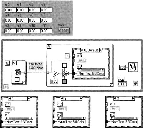
Suppose you wanted to display hundreds of numbers simultaneously from your DAQ experiment. You could use the Multicolumn Listbox or Table indicator (from Controls»List & Table) if you really want to maximize your use of front panel real estate. To build a grid of numbers in which you can control the color of each number in order to indicate an alarm condition, create the VI shown in Figure 6–63 using these tips:

1.   First, drop only one Simple Numeric control from the Functions»Classic Controls palette—I chose this one to optimize screen area. Change it to an indicator. Label it “n 0” so that when we begin cloning, the numbering will happen automatically—this would not work if we had used the label “n0”.

2.   Create a Property Node for “n 0” and change its property to the one shown in the figure (use its Properties»Numeric Text»Text Colors»BG Color pop-up menu item). Make this Property Node a “write” node with its Change All To Write pop-up menu item.

3.   To most efficiently create 11 copies of our numeric indicator and its Property node, we cannot clone them. Instead, select both nodes on the block diagram, then copy and paste them repeatedly (<Ctrl-C>, click where you want the copy, then <Ctrl-V>).

4.   The two boxes connected to the Select function are Color Box constants from the Functions»Numeric»Additional Numeric Constants palette. Using your Coloring tool and Color Copying tool , color the top one the same gray color as the front panel, and the bottom one white.

5.  The Case Structure has 12 cases wired just like the three shown in Figure 6–63.

Run the VI and see how the alarm conditions are shown.

6.6.3 Speeding Up Graphs (or Charts)

Compared to many other common front panel items, graphs and charts take a long time to display. Here are a number of techniques for speeding them up:

Figure 6–63
Many numeric values are shown.

1.   Get a faster computer or a faster video card.

2.   Make your graph smaller. The time required to update a graph is roughly proportional to the area of the graph.

3.   If the graph is a chart, you can set its update mode with its popup menu item Advanced»Update Mode. The slowest update mode by far is Strip Chart, and the fastest is Sweep Chart.

4.   Do not have other front panel objects overlapping the graph.

5.   Turn off autoscaling if it’s not needed.

6.   Only update the graph every N iterations of its enclosing loop with a Case Structure. The graph will still take just as long to draw whenever it does.

7.   If the technique in step 6 interferes with your DAQ timing whenever the graph is drawn, you can use two White Loops running simultaneously. One loop has the graph, and the other has the DAQ operations implemented as a subVI with a high priority (via File»VI Properties»Category»Execution»Priority). This priority business is a very inexact science, so you’ll need to experiment with it! You’ll also need to use a local or global to get your data from the DAQ loop to the graph loop, and this can be tricky.

6.7 ALARMS

Visible or audible alarms will let you know if something is going wrong with your DAQ project, and there are many ways to implement them.

6.7.1 Visible Alarms

The simplest way to create visible alarm on a front panel is to set a big Boolean indicator to True, where True is a noticeable color. Flashing this indicator makes it even more noticeable. The second simplest method, if your front panel is already crowded (as most are), is to change the color of an existing very large control (or controls). The third simplest method is to show a dialog box. If you must still perform DAQ when this dialog box is showing, things become less simple; refer to Section 6.1.4 if you want to try this.

There is still no way to programmatically change the color of your front panel. You can, however, create a giant Boolean indicator that covers the entire background of your front panel to simulate such a thing. Another more effective approach is to use a digital output on your DAQ device to drive a relay that drives a bright flashing light. This is appropriate for noisy industrial environments or whenever the operator may not be able to see the monitor.

6.7.2 Audible Alarms

The simplest audible alarm is to use the computer’s sound card to play WAV files, or some other sound file, through common amplified speakers connected to your computer. The Functions»Graphics & Sound palette has functions that can handle this. There are a number of disadvantages to this sound card approach:

1.   Your computer’s sound driver might become disabled at any time without your knowledge. For example, if somebody opens up another application that uses the sound driver, or sometimes even if your operating system is running very low on memory, LabVIEW might be unable to use it.

2.   Somebody might turn down the speaker’s volume.

3.   Somebody might switch off the amplifier’s power supply.

A more reliable approach is to use a digital output on your DAQ device to drive a relay that drives another audible alarm, such as a buzzer or loud siren. See Chapter 8, Section 8.2.2 if your DAQ device doesn’t have any spare digital I/O.

6.7.3 Paging Techniques

There exist a number of modem-driving utilities on various Web sites that you can use to send a message to a pager. Sending an alphanumeric message can be especially helpful, as text is more descriptive than numbers. Sometimes you cannot connect to an analog telephone (for modem driver reasons), or you might have no access to any phone line at all (for security reasons). It is possible to use LabVIEW to send an email that will relay a message to a pager. You’re on your own when it comes to implementing this, as this will vary per company, but NI’s Internet Developers Toolkit (G Web Server) makes emailing from LabVIEW easy. If you work at a company with network-savvy staff, they will already know how to reliably send an email that will activate a pager.

6.8 POWER LOSSES

Your computer may lose power for any number of reasons. Since this could happen white your DAQ experiment is running, you may want to consider taking the necessary steps to automatically continue your experiment in the event of power loss. Here are issues to consider:

1.   For lengthy experiments, you will need to write your program so that it expects to automatically resume upon power up. To do this, you will need to occasionally write the status of your test to disk white the experiment is running, as the disk will likely be the only place with any data remaining when the power comes back on. Everything in memory, like shift registers and global variables, not to mention your entire LabVIEW program, is immediately terminated when your computer powers down.

2.   If you’re running Windows, you can place a shortcut to your VI in Windows’ startup folder so it will start itself upon power up. This folder is typically something like C:WindowsStart MenuProgramsStartUp. A similar mechanism can be implemented on all non-Windows LabVIEW-compatible platforms.

3.   You will want to use item 15 in Appendix E.

4.   If your computer has dialog boxes that pop up and prevent LabVIEW from running during power up, you will need to figure out some way to get rid of these boxes. The usual such dialog box is the networking login box. If you’re running Windows, Microsoft was kind enough to offer TweakUI, which can automatically log you in when this networking box shows up. Search the Web using a search engine to find TweakUI; it has a habit of moving around frequently, as does everything else on Microsoft’s Web site. This has security consequences, of course.