
Chapter 8: Programming Distance Sensors with Python
In this chapter, we look at distance sensors and how to use them to avoid objects. Avoiding obstacles is a key feature in mobile robots, as bumping into stuff is generally not good. It is also a behavior that starts to make a robot appear smart, as if it is behaving intelligently.
In this chapter, we find out about the different types of sensors and choose a suitable type. We then build a layer in our robot object to access them and, in addition to this, we create a behavior to avoid walls and objects.
You will learn about the following topics in this chapter:
- Choosing between optical and ultrasonic sensors
- Attaching and reading an ultrasonic sensor
- Avoiding walls – writing a script to avoid obstacles
Technical requirements
To complete the hands-on experiments in this chapter, you will require the following:
- The Raspberry Pi robot and the code from the previous chapters.
- Two HC-SR04P, RCWL-1601, or Adafruit 4007 ultrasonic sensors. They must have a 3.3 V output.
- A breadboard.
- 22 AWG single-core wire or a pre-cut breadboard jumper wire kit.
- A breadboard-friendly single pole, double toggle (SPDT) slide switch.
- Male-to-female jumpers, preferably of the joined-up jumper jerky type.
- Two brackets for the sensor.
- A crosshead screwdriver.
- Miniature spanners or small pliers.
The code for this chapter is available on GitHub at https://github.com/PacktPublishing/Learn-Robotics-Programming-Second-Edition/tree/master/chapter8.
Check out the following video to see the Code in Action: https://bit.ly/2KfCkZM
Choosing between optical and ultrasonic sensors
Before we start to use distance sensors, let's find out what these sensors actually are, how they work, and some of the different types available.
The most common ways in which to sense distance are to use ultrasound or light. The principle of both of these mechanisms is to fire off a pulse and then sense its reflected return, using either its timing or angle to measure a distance, as can be seen in the following diagram:
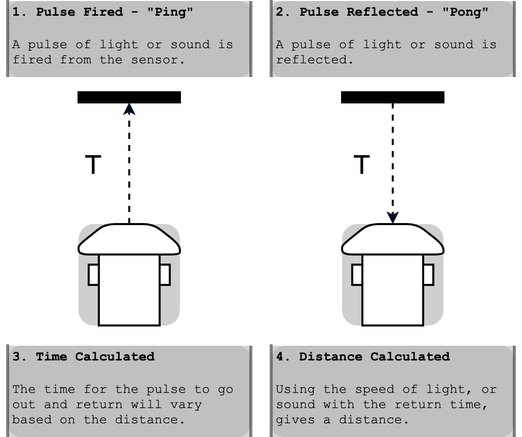
Figure 8.1 – Using pulse timing in a distance sensor
We focus on the sensors that measure the response time, otherwise known as the time of flight. Figure 8.1 shows how these sensors use reflection time.
With this basic understanding of how sensors work, we'll now take a closer look at optical sensors and ultrasonic sensors.
Optical sensors
Light-based sensors, like the one in Figure 8.2, use infrared laser light that we cannot see. These devices can be tiny; however, they can suffer in strong sunlight and fluorescent light, making them misbehave. Some objects reflect light poorly or are transparent and are undetectable by these sensors:
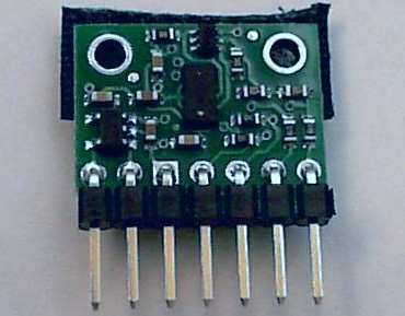
Figure 8.2 – A VL530LOx on a carrier board
In competitions where infrared beams detect course times, the beams and these sensors can interfere with each other. However, unlike ultrasonic sensors, these are unlikely to cause false detections when placed on different sides of a robot. Optical distance sensors can have higher accuracy, but over a more limited range. They can be expensive, although there are cheaper fixed range types of light sensors out there.
Ultrasonic sensors
Many sound-based distance measuring devices use ultrasonic sound with frequencies beyond human hearing limits, although they can annoy some animals, including dogs. Mobile phone microphones and some cameras pick up their pulses as clicks. Ultrasonic devices tend to be larger than optical ones, but cheaper since sound travels slower than light and is easier to measure. Soft objects that do not reflect sound, such as fabrics, can be harder for these to detect.
Figure 8.3 shows the HC-SR04, a common and inexpensive sound-based distance sensor:
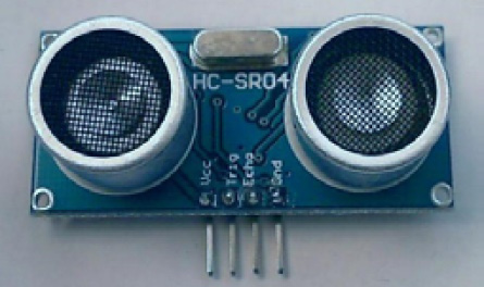
Figure 8.3 – The HC-SR04
They have a range of up to 4 meters from a minimum of about 2 cm.
There are a number of ultrasonic-based devices, including the common HC-SR04, but not all of them are suitable. We'll look at logic levels as this is an important factor in choosing which sensor to buy.
Logic levels and shifting
The I/O pins on the Raspberry Pi are only suitable for inputs of 3.3 V. Many devices in the market have a 5 V logic, either for their inputs when controlling them, or from their outputs. Let's dig into what I mean by logic levels, and why it is sensible to try and stick to the native voltage level when possible.
Voltage is a measure of how much pushing energy there is on an electrical flow. Different electronics are built to tolerate or to respond to different voltage levels. Putting too high a voltage through a device can damage it. On the other hand, putting too low a voltage can cause your sensors or outputs to simply not respond or behave strangely. We are dealing with logic devices that output a high or low voltage to represent a true/false value. These voltages must be above a threshold to be true, and below it to be false. We must be aware of these electrical properties, or we will destroy things and fail to get them to communicate.
The graph in Figure 8.4 shows the effects that different levels have:
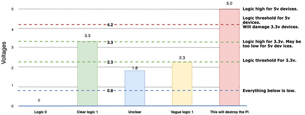
Figure 8.4 – Voltages and logic levels
In Figure 8.4, we show a graph. On the y-axis (left), it shows voltage labels from 0 to 5 V. The y-axis shows different operating conditions. There are 4 dashed lines running through the graph. The lowest dashed line is at 0.8 V; below this, an input will consider it as logic 0. The next line, at around 2.3 V, is where many 3.3 V devices consider things at logic 1. The line at 3.3 V shows the expected input and output level for logic 1 on a Raspberry Pi. Above this line, damage may occur to a Raspberry Pi. At around 4.2 V is what some 5 V devices expect for logic 1 (although some will allow as low as 2 V for this) – the Raspberry Pi needs help to talk to those.
Along the graph are 5 bars. The first labeled bar is at 0 – meaning a clear logic 0 to all devices. The next bar is a clear logic 1 for the Raspberry Pi at 3.3 V, but it is also below 4.2 V, so some 5 V devices won't recognize this. The bar labelled unclear is at 1.8 V – in this region, between the low and the high thresholds, the logic might not be clear, and this should be avoided. The bar labeled Vague logic 1 is above the threshold, but only just, and could be misinterpreted or cause odd results on 3.3 V devices. The last bar is at 5 V, which 5 V devices output. This must not go to the Raspberry Pi without a level shifter or it will destroy that Raspberry Pi.
There are bars in Figure 8.4 at 1.7 V and 2.3 V. These voltages are very close to the logic threshold and can result in random data coming from the input. Avoid intermediate voltages between the required logic levels. 3 V is OK, but avoid 1.5 V as this is ambiguous.
Important note
Putting more than 3.3 V into a Raspberry Pi pin damages the Raspberry Pi. Do not use 5 V devices without logic level shifters.
If you use devices that are 5 V, you require extra electronics to interface them. The electronics come with further wiring and parts, thereby increasing the cost, complexity, or size of the robot's electronics:

Figure 8.5 – Wiring the HC-SR04 sensors into the level shifters
Figure 8.5 shows a wiring diagram for a robot that uses HC-SR04 5v sensors that require logic level shifting. This circuit diagram shows the Raspberry Pi GPIO pins at the top. Coming from 3 pins to the left are the 5 V, 3.3 V (written as 3v3), and ground (GND) lines. Below the GPIO pins are the 3.3 V and 5 V lines.
Below the power lines (or rails) are two level shifters. Going into the right of the level shifters are connections from the Raspberry Pi GPIO pins 5, 6, 17, and 27. In this style of diagram, a black dot shows a connection, and lines that do not connect are shown with a bridge.
The bottom of the diagram has a ground line from the ground pin. This is shown as it's normal that additional electronics will require access to a ground line.
The left of the diagram has the two distance sensors, with connections to 5 V and GND. Each sensor has the trig and echo pins wired to the level shifters. It's not hard to see how adding more sensors that also require level shifters to this would further increase complexity.
Thankfully, other options are now available. Where it is possible to use a 3.3 V native device or a device that uses its supply voltage for logic high, it is worth choosing these devices. When buying electronics for a robot, consider carefully what voltage the robot's main controller uses (like the Raspberry Pi), and check that the electronics work with the controller's voltages.
The HC-SR04 has several replacement parts that have this ability. The HC-SR04P, the RCWL-1601, and Adafruit 4007 models output 3.3 V and can connect directly to the Raspberry Pi.
Why use two sensors?
Having two sensors allows a behavior to detect which side is closer. With this, the robot can detect where open spaces are and move toward them. Figure 8.6 shows how this works:
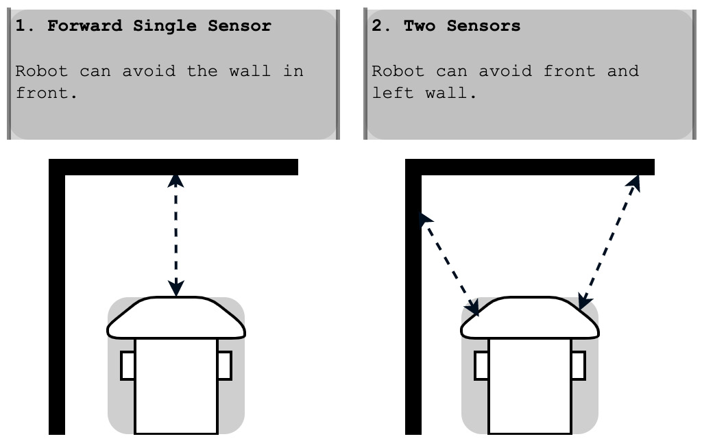
Figure 8.6 – Using two sensors
In Figure 8.6, the second robot can make more interesting decisions because it has more data from the world with which to make those decisions.
Considering all of these options, I recommend you use a 3.3 V variant like the HC-SR04P/RCWL-1601 or Adafruit 4007 because they are cheap and because it is easy to add two or more of these sensors.
We've seen some distance sensor types and discussed the trade-offs and choices for this robot. You've learned about voltage levels, and why this is a crucial consideration for robot electronics. We've also looked at how many sensors we could use and where we could put them. Now let's look at how to add them.
Attaching and reading an ultrasonic sensor
First, we should wire in and secure these sensors to the robot. We then write some simple test code that we can use to base our behavior code on in the next section. After completing this section, the robot block diagram should look like Figure 8.7:
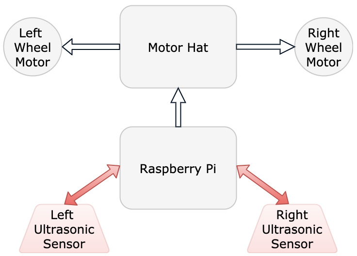
Figure 8.7 – Robot block diagram with ultrasonic sensors
This diagram builds on the block diagram in Figure 6.33 from Chapter 6, Building Robot Basics – Wheels, Power, and Wiring by adding left and right ultrasonic sensors. Both have bi-directional arrows to the Raspberry Pi, since, being an active sensor, the Raspberry Pi triggers a sensor measurement and then reads back the result. Let's attach the sensors to the robot chassis.
Securing the sensors to the robot
In the Technical requirements section, I added an HC-SR04 bracket. Although it is possible to make a custom bracket with CAD and other part making skills, it is more sensible to use one of the stock designs. Figure 8.8 shows the bracket I'm using:
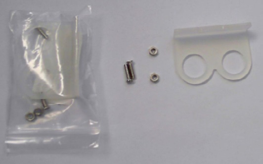
Figure 8.8 – Ultrasonic HC-SR04 sensor brackets with the screws and hardware
These are easy to attach to your robot, assuming that your chassis is similar enough to mine, in that it has mounting holes or a slot to attach this bracket:

Figure 8.9 – Steps for mounting the sensor bracket
To mount the sensor bracket, use Figure 8.9 as a guide for the following steps:
- Push the two bolts into the holes on the bracket.
- Push the bracket screws through the holes at the front of the robot.
- Thread a nut from underneath the robot on each and tighten. Repeat this for the other side.
- The robot should look like this with the two brackets mounted.
Figure 8.10 shows how to push the sensors into the brackets:

Figure 8.10 – Pushing the sensors into the brackets
- Look at the sensor. The two transducer elements, the round cans with a gauze on top, will fit well in the holes in the brackets.
- The distance sensors can simply be pushed into the brackets, since they have a friction fit. The electrical connector for the sensor should be facing upward.
- After putting in both sensors, the robot should look like panel 7 of Figure 8.10.
You've now attached the sensors to the chassis. Before we wire them, we'll take a slight detour and add a helpful power switch.
Adding a power switch
Before we turn on the robot again, let's add a switch for the motor power. This switch is more convenient than screwing the ground wire from the battery into the terminal repeatedly. We'll see how to do this in three simple steps. Follow along:
- Make sure you have the following equipment ready, as shown in Figure 8.11: a breadboard, some velcro, a mini breadboard-friendly SPDT switch, and one length of single-core 22 AWG wire:

Figure 8.11 – Items needed to add a power switch
- Now use two strips of Velcro to stick the breadboard on top of the robot's battery, as shown in Figure 8.12. The velcro holds firm but is easy to remove if you need to disassemble the robot:

Figure 8.12 – Adding velcro strips
With the breadboard in place, we can now add a switch.
Take a look at Figure 8.13 for details on how the switch is connected:
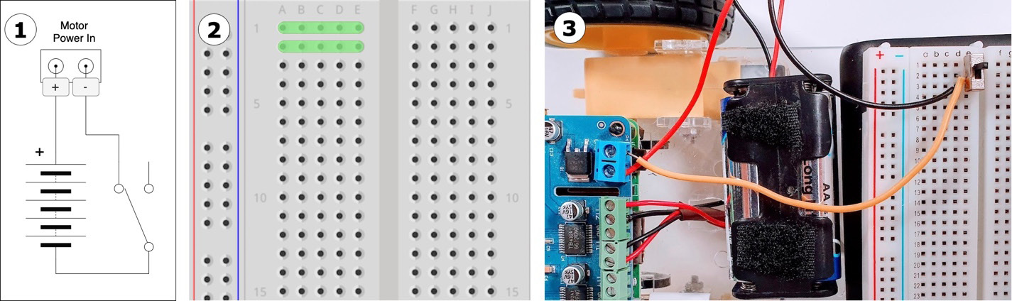
Figure 8.13 – Wiring the switch
Figure 8.13 shows a circuit diagram, a close-up of a breadboard, and a suggested way to wire the physical connections on the robot. Let's look at this in detail:
- This is a circuit diagram showing the batteries, switch, and motor power input connectors. At the top is the motor power in terminal. From the positive (+) side of that terminal, a wire goes down the left to the batteries, shown as alternating thick and thin bars. From the batteries, the bottom terminal is their negative side. A wire goes from this around to the switch on the right of the diagram. The top of the switch is then connected via a wire to the negative (-) side of the motor power in terminal. This is the important diagram for making the connections.
- Before we physically wire the switch, it's worth talking about the rows of the breadboard. This panel shows a close-up of a breadboard, with 2 of the rows highlighted in green lines. The green lines show that the rows are connected in groups of 5. The arrangement of a breadboard has two wired groups of 5 holes (tie-points) for each of the rows (numbered 1 to 30). It has a groove in the middle separating the groups.
- The physical wiring uses the breadboard to make connections from wires to devices. It won't match the diagram precisely. The left shows the motor board, with a red wire from the batteries, their positive side, going into the positive (+ or VIN) terminal on the motor power in terminal. The batteries are in the middle. A black wire goes from the batteries into the breadboard in row 3, column d. In column e, a switch is plugged into the breadboard going across rows 1, 2, and 3. An orange precut 22 AWG wire goes from row 2 to the GND terminal, where it is screwed in. Sliding this switch turns on the power to the robot motors.
We've now given our robot a power switch for its motor batteries, so we can turn the motor power on without needing a screwdriver. Next, we will use the same breadboard to wire up the distance sensors.
Wiring the distance sensors
Each ultrasonic sensor has four connections:
- A trigger pin to ask for a reading
- An echo pin to sense the return
- A VCC/voltage pin that should be 3.3 V
- A GND or ground pin
Ensure that the whole robot is switched off before proceeding any further. The trigger and echo pins need to go to GPIO pins on the Raspberry Pi.
Figure 8.14 shows a close-up of the Raspberry Pi GPIO port to assist in making connections:

Figure 8.14 – Raspberry Pi connections
Figure 8.14 is a diagram view of the GPIO connector on the Raspberry Pi. This connector is the 40 pins set in two rows at the top of the Pi. Many robots and gadgets use them. The pin numbers/names are not printed on the Raspberry Pi, but this diagram should assist in finding them.
We use a breadboard for this wiring. Figure 8.15 shows the connections needed for these:

Figure 8.15 – Sensor wiring diagram
Wires from the Raspberry Pi to the breadboard, and from the sensor to the breadboard, need male-to-female jumper wires. Wires on the breadboard (there are only 4 of these) use short pre-cut wires. Figure 8.15 shows a circuit diagram above, and a breadboard wiring suggestion below.
To wire the sensors, use Figure 8.15 as a guide, along with these steps:
- Start with the power connections. A wire goes from the 3.3 V (often written as 3v3 on diagrams) pin on the Raspberry Pi to the top, red-marked rail on the breadboard. We can use this red rail for other connections needing 3.3 V.
- A wire from one of the GND pins on the Pi goes to the black- or blue-marked rail on the breadboard. We can use this blue rail for connections requiring GND.
- Pull off a strip of 4 from the male-to-female jumper wires for each side.
- For the left-hand sensor, identify the four pins—VCC, trig, echo, and GND. For the connection from this to the breadboard, it's useful to keep the 4 wires together. Take 4 male-to-female connectors (in a joined strip if possible), from this sensor, and plug them into the board.
- On the breadboard, use the precut wires to make a connection from ground to the blue rail, and from VCC to the red rail.
- Now use some jumper wires to make the signal connections from the trig/echo pins to the Raspberry Pi GPIO pins.
Important note
Depending on where you've placed your breadboard, the distance sensor wires may not reach. If this is the case, join two male-to-female wires back to back, and use some electrical tape to bind them together.
For neatness, I like to wrap wires in spiral wrap; this is entirely optional but can reduce the clutter on the robot.
Please double-check your connections before you continue. You have now installed the distance sensors into your robot's hardware, but in order to test and use them, we need to prepare the software components.
Installing Python libraries to communicate with the sensor
To work with the GPIO sensor, and some other hardware, you need a Python library. Let's use the GPIOZero library, designed to help interface with hardware like this:
$ pip3 install RPi.GPIO gpiozero
With the library now installed, we can write our test code.
Reading an ultrasonic distance sensor
To write code for distance sensors, it helps to understand how they work. As suggested previously, this system works by bouncing sound pulses off of objects and measuring the pulse return times.
The code on the Raspberry Pi sends an electronic pulse to the trigger pin to ask for a reading. In response to this pulse, the device makes a sound pulse and times its return. The echo pin responds using a pulse too. The length of this pulse corresponds to the sound travel time.
The graph in Figure 8.16 shows the timing of these:
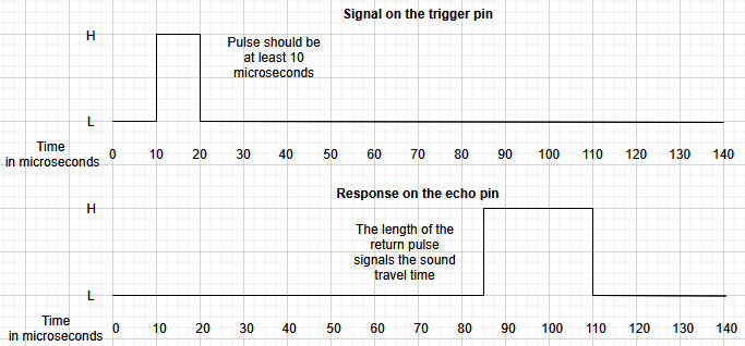
Figure 8.16 – Timing of a pulse and the response for an ultrasonic distance sensor
The GPIOZero library can time this pulse, and convert it into a distance, which we can use in our code.
The device might fail to get a return response in time if the sound didn't echo back soon enough. Perhaps the object was outside the sensor's range, or something dampened the sound.
As we did with our servo motor control class previously, we should use comments and descriptive names to help us explain this part of the code. I've called this file test_distance_sensors.py:
- Begin by importing time and the DistanceSensor library:
import time
from gpiozero import DistanceSensor
- Next, we set up the sensors. I've used print statements to show what is going on. In these lines, we create library objects for each distance sensor, registering the pins we have connected them on. Try to make sure these match your wiring:
print("Prepare GPIO Pins")
sensor_l = DistanceSensor(echo=17, trigger=27, queue_len=2)
sensor_r = DistanceSensor(echo=5, trigger=6, queue_len=2)
You'll note the extra queue_len parameter. The GPIOZero library tries to collect 30 sensor readings before giving an output, which makes it smoother, but less responsive. And what we'll need for our robot is responsive, so we take it down to 2 readings. A tiny bit of smoothing, but totally responsive.
- This test then runs in a loop until we cancel it:
while True:
- We then print the distance from our sensors. .distance is a property, as we saw with the .count property on our LED system earlier in the book. The sensors are continuously updating it. We multiply it by 100 since GPIOZero distance is in terms of a meter:
print("Left: {l}, Right: {r}".format(
l=sensor_l.distance * 100,
r=sensor_r.distance * 100))
- A little sleep in the loop stops it flooding the output too much and prevents tight looping:
time.sleep(0.1)
- Now, you can turn on your Raspberry Pi and upload this code.
- Put an object anywhere between 4 centimeters and 1 meter away from the sensor, as demonstrated in the following image:

Figure 8.17 – Distance sensor with object
Figure 8.17 shows an item roughly 10.5 cm from a sensor. The object is a small toolbox. Importantly it is rigid and not fabric.
- Start the code on the Pi with python3 test_distance_sensors.py. As you move around the object, your Pi should start outputting distances:
pi@myrobot:~ $ python3 test_distance_sensors.py
Prepare GPIO Pins
Left: 6.565688483970461, Right: 10.483658125707734
Left: 5.200715097982538, Right: 11.58136928065528
- Because it is in a loop, you need to press Ctrl + C to stop the program running.
- You'll see here that there are many decimal places, which isn't too helpful here. First, the devices are unlikely to be that accurate, and second, our robot does not need sub-centimeter accuracy to make decisions. We can modify the print statement in the loop to be more helpful:
print("Left: {l:.2f}, Right: {r:.2f}".format(
l=sensor_l.distance * 100,
r=sensor_r.distance * 100))
:.2f changes the way text is output, to state that there are always two decimal places. Because debug output can be essential to see what is going on in the robot, knowing how to refine it is a valuable skill.
- Running the code with this change gives the following output:
pi@myrobot:~ $ python3 test_distance_sensors.py
Prepare GPIO Pins
Left: 6.56, Right: 10.48
Left: 5.20, Right: 11.58
You've demonstrated that the distance sensor is working. Added to this is exploring how you can tune the output from a sensor for debugging, something you'll do a lot more when making robots. To make sure you're on track, let's troubleshoot anything that has gone wrong.
Troubleshooting
If this sensor isn't working as expected, try the following troubleshooting steps:
- Is anything hot in the wiring? Hold the wires to the sensor between the thumb and forefinger. Nothing should be hot or even warming! If so, remove the batteries, turn off the Raspberry Pi, and thoroughly check all wiring against Figure 8.12.
- If there are syntax errors, please check the code against the examples. You should have installed Python libraries with pip3 and be running with python3.
- If you are still getting errors, or invalid values, please check the code and indentation.
- If the values are always 0, or the sensor isn't returning any values, then you may have swapped trigger and echo pins. Try swapping the trigger/echo pin numbers in the code and testing it again. Don't swap the cables on a live Pi! Do this one device at a time.
- If you are still getting no values, ensure you have purchased 3.3 V-compatible systems. The HC-SR04 model will not work with the bare Raspberry Pi.
- If values are way out or drifting, then ensure that the surface you are testing on is hard. Soft surfaces, such as clothes, curtains, or your hand, do not respond as well as glass, wood, metal, or plastic. A wall works well!
- Another reason for incorrect values is the surface may be too small. Make sure that your surface is quite wide. Anything smaller than about 5 cm square may be harder to measure.
- As a last resort, if one sensor seems fine, and the other wrong, it's possible that a device is faulty. Try swapping the sensors to check this. If the result is different, then a sensor may be wrong. If the result is the same, it is the wiring or code that is wrong.
You have now troubleshooted your distance sensor and made sure that it works. You have seen it output values to show that it is working and tested it with objects to see its response. Now, let's step up and write a script to avoid obstacles.
Avoiding walls – writing a script to avoid obstacles
Now that we have tested both sensors, we can integrate them with our robot class and make obstacle avoidance behavior for them. This behavior loop reads the sensors and then chooses behavior accordingly.
Adding the sensors to the robot class
So, before we can use the sensors in a behavior, we need to add them to the Robot class, assigning the correct pin numbers for each side. This way, if pin numbers change or even the interface to a sensor changes, behaviors will not need to change:
- To use the DistanceSensor object, we need to import it from gpiozero; the new code is in bold:
from Raspi_MotorHAT import Raspi_MotorHAT
from gpiozero import DistanceSensor
- We create an instance of one of these DistanceSensor objects for each side in the robot class. We need to set these up in the constructor for our robot. We use the same pin numbers and queue length as in our test:
class Robot:
def __init__(self, motorhat_addr=0x6f):
# Setup the motorhat with the passed in address
self._mh = Raspi_MotorHAT(addr=motorhat_addr)
# get local variable for each motor
self.left_motor = self._mh.getMotor(1)
self.right_motor = self._mh.getMotor(2)
# Setup The Distance Sensors
self.left_distance_sensor = DistanceSensor(echo=17, trigger=27, queue_len=2)
self.right_distance_sensor = DistanceSensor(echo=5, trigger=6, queue_len=2)
# ensure the motors get stopped when the code exits
atexit.register(self.stop_all)
Adding this to our robot layer makes it available to behaviors. When we create our robot, the sensors will be sampling distances. Let's make a behavior that uses them.
Making the obstacle avoid behaviors
This chapter is all about getting a behavior; how can a robot drive and avoid (most) obstacles? The sensor's specifications limit it, with smaller objects or objects with a soft/fuzzy shell, such as upholstered items, not being detected. Let's start by drawing what we mean in Figure 8.18:
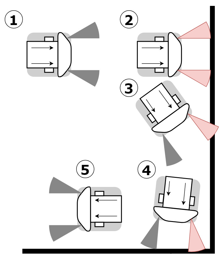
Figure 8.18 – Obstacle avoidance basics
In our example (Figure 8.18), a basic robot detects a wall, turns away, keeps driving until another wall is detected, and then turns away from that. We can use this to make our first attempt at wall-avoiding behavior.
First attempt at obstacle avoidance
To help us understand this task, the following diagram shows a flow diagram for the behavior:

Figure 8.19 – Obstacle avoidance flowchart
The flow diagram in Figure 8.19 starts at the top.
This diagram describes a loop that does the following:
- The Start box goes into a Get Distances box, which gets the distances from each sensor.
- We test whether the left sensor reads less than 20 cm (a reasonable threshold):
a) If so, we set the left motor in reverse to turn the robot away from the obstacle.
b) Otherwise, we drive the left motor forward.
- We now check the right sensor, setting it backward if closer than 20 cm, or forward if not.
- The program waits a short time and loops around again.
We put this loop in a run method. There›s a small bit of setup required in relation to this. We need to set the pan and tilt to 0 so that it won't obstruct the sensors. I've put this code in simple_avoid_behavior.py:
- Start by importing the robot, and sleep for timing:
from robot import Robot
from time import sleep
...
- The following class is the basis of our behavior. There is a robot object stored in the behavior. A speed is set, which can be adjusted to make the robot go faster or slower. Too fast, and it has less time to react:
...
class ObstacleAvoidingBehavior:
"""Simple obstacle avoiding"""
def __init__(self, the_robot):
self.robot = the_robot
self.speed = 60
...
- Now the following method chooses a speed for each motor, depending on the distance detected by the sensor. A nearer sensor distance turns away from the obstacle:
...
def get_motor_speed(self, distance):
"""This method chooses a speed for a motor based on the distance from a sensor"""
if distance < 0.2:
return -self.speed
else:
return self.speed
...
- The run method is the core, since it has the main loop. We put the pan and tilt mechanism in the middle so that it doesn't obstruct the sensors:
...
def run(self):
self.robot.set_pan(0)
self.robot.set_tilt(0)
- Now, we start the main loop:
while True:
# Get the sensor readings in meters
left_distance = self.robot.left_distance_sensor.distance
right_distance = self.robot.right_distance_sensor.distance
...
- We then print out our readings on the console:
...
print("Left: {l:.2f}, Right: {r:.2f}".format(l=left_distance, r=right_distance))
...
- Now, we use the distances with our get_motor_speed method and send this to each motor:
...
# Get speeds for motors from distances
left_speed = self.get_motor_speed(left_distance)
self.robot.set_left(left_speed)
right_speed = self.get_motor_speed(right_distance)
self.robot.set_right(right_speed)
- Since this is our main loop, we wait a short while before we loop again. Under this is the setup and starting behavior:
...
# Wait a little
sleep(0.05)
bot = Robot()
behavior = ObstacleAvoidingBehavior(bot)
behavior.run()
The code for this behavior is now completed and ready to run. It's time to try it out. To test this, set up a test space to be a few square meters wide. Avoid obstacles that the sensor misses, such as upholstered furniture or thin obstacles such as chair legs. I've used folders and plastic toy boxes to make courses for these.
Send the code to the robot and try it out. It drives until it encounters an obstacle, and then turns away. This kind of works; you can tweak the speeds and thresholds, but the behavior gets stuck in corners and gets confused.
Perhaps it's time to consider a better strategy.
More sophisticated object avoidance
The previous behavior can leave the robot stuck. It appears to be indecisive with some obstacles and occasionally ends up ramming others. It may not stop in time or turn into things. Let's make a better one that drives more smoothly.
So, what is our strategy? Well, let's think in terms of the sensor nearest to an obstacle, and the furthest. We can work out the speeds of the motor nearest to it, the motor further from it, and a time delay. Our code uses the time delay to be decisive about turning away from a wall, with the time factor controlling how far we turn. This reduces any jitter. Let's make some changes to the last behavior for this:
- First, copy the simple_avoid_behavior.py file into a new file called avoid_behavior.py.
- We won't be needing get_motor_speed, so remove that. We replace it with a function called get_speeds. This takes one parameter, nearest_distance, which should always be the distance sensor with the lower reading:
...
def get_speeds(self, nearest_distance):
if nearest_distance >= 1.0:
nearest_speed = self.speed
furthest_speed = self.speed
delay = 100
elif nearest_distance > 0.5:
nearest_speed = self.speed
furthest_speed = self.speed * 0.8
delay = 100
elif nearest_distance > 0.2:
nearest_speed = self.speed
furthest_speed = self.speed * 0.6
delay = 100
elif nearest_distance > 0.1:
nearest_speed = -self.speed * 0.4
furthest_speed = -self.speed
delay = 100
else: # collison
nearest_speed = -self.speed
furthest_speed = -self.speed
delay = 250
return nearest_speed, furthest_speed, delay
...
These numbers are all for fine-tuning. The essential factor is that depending on the distance, we slow down the motor further from the obstacle, and if we get too close, it drives away. Based on the time delay, and knowing which motor is which, we can drive our robot.
- Most of the remaining code stays the same. This is the run function you've already seen:
...
def run(self):
# Drive forward
self.robot.set_pan(0)
self.robot.set_tilt(0)
while True:
# Get the sensor readings in meters
left_distance = self.robot.left_distance_sensor.distance
right_distance = self.robot.right_distance_sensor.distance # Display this
self.display_state(left_distance, right_distance)
...
- It now uses the get_speeds method to determine a nearest and furthest distance. Notice that we take the min, or minimum, of the two distances. We get back the speeds for both motors and a delay, and then print out the variables so we can see what's going on:
...
# Get speeds for motors from distances
nearest_speed, furthest_speed, delay = self.get_speeds(min(left_distance, right_distance))
print(f"Distances: l {left_distance:.2f}, r {right_distance:.2f}. Speeds: n: {nearest_speed}, f: {furthest_speed}. Delay: {delay}")
...
We've used an f-string here, a further shortcut from .format (which we used previously). Putting the letter prefix f in front of a string allows us to use local variables in curly brackets in the string. We are still able to use .2f to control the number of decimal places.
- Now, we check which side is nearer, left or right, and set up the correct motors:
...
# Send this to the motors
if left_distance < right_distance:
self.robot.set_left(nearest_speed)
self.robot.set_right(furthest_speed)
else:
self.robot.set_right(nearest_speed)
self.robot.set_left(furthest_speed)
...
- Instead of sleeping a fixed amount of time, we sleep for the amount of time in the delay variable. The delay is in milliseconds, so we need to multiply it to get seconds:
...
# Wait our delay time
sleep(delay * 0.001)
...
- The rest of the code remains the same. You can find the full code for this file at https://github.com/PacktPublishing/Learn-Robotics-Programming-Second-Edition/tree/master/chapter8.
When you run this code, you should see smoother avoidance. You may need to tweak the timings and values. The bottom two conditions, reversing and reverse turning, might need to be tuned. Set the timings higher if the robot isn't quite pulling back enough, or lower if it turns away too far.
There are still flaws in this behavior, though. It does not construct a map at all and has no reverse sensors, so while avoiding objects in front, it can quite quickly reverse into objects behind it. Adding more sensors could resolve some of these problems. Still, we cannot construct a map just yet as our robot does not have the sensors to determine how far it has turned or traveled accurately.
Summary
In this chapter, we have added sensors to our robot. This is a major step as it makes the robot autonomous, behaving on its own and responding in some way to its environment. You've learned how to add distance sensing to our robots, along with the different kinds of sensors that are available. We've seen code to make it work and test these sensors. We then created behaviors to avoid walls and looked at how to make a simplified but flawed behavior, and how a more sophisticated and smoother behavior would make for a better system.
With this experience, you can consider how other sensors could be interfaced with your robot, and some simple code to interact with them. You can output data from sensors so you can debug their behavior and create a behavior to make a robot perform some simple navigation on its own.
In the next chapter, we look further into driving predetermined paths and straight lines using an encoder to make sure that the robot moves far more accurately. We use an encoder to compare our motor's output with our expected goals and get more accurate turns.
Exercises
- Some robots get by with just a single sensor. Can you think of a way of avoiding obstacles reliably with a single sensor?
- We have a pan/tilt mechanism, which we use later for a camera. Consider putting a sensor on this, and how to incorporate this into a behavior.
- The robot behavior we created in this chapter can reverse into things. How could you remedy this? Perhaps make a plan and try to build it.
Further reading
Please refer to the following links for more information:
- The RCWL-1601 is still quite similar to the HC-SR04. The HC-SR04 data sheet has useful information about its range. You can find the data sheet at https://www.mouser.com/ds/2/813/HCSR04-1022824.pdf.
- ModMyPi has a tutorial with an alternative way to wire the original HC-SR04 types, and level shift their IO: https://www.modmypi.com/blog/hc-sr04-ultrasonic-range-sensor-on-the-raspberry-pi.
- Raspberry Pi Tutorials also has a breadboard layout and Python script, using RPi.GPIO instead of gpiozero, at https://tutorials-raspberrypi.com/raspberry-pi-ultrasonic-sensor-hc-sr04/.
- We've started to use many pins on the Raspberry Pi. When trying to ascertain which pins to use, I highly recommend visiting the Raspberry Pi GPIO at https://pinout.xyz/.
- We briefly mentioned debug output and refining it. W3schools has an interactive guide to Python format strings at https://www.w3schools.com/python/ref_string_format.asp.
- There are many scholarly articles available on more interesting or sophisticated object behavior. I recommend reading Simple, Real-Time Obstacle Avoidance Algorithm (https://pdfs.semanticscholar.org/519e/790c8477cfb1d1a176e220f010d5ec5b1481.pdf) for mobile robots for a more in-depth look at these behaviors.