
The previous chapter showed how to use the Elastic stack for a business (logging) use case, which confirms that Elastic is not only a solution made for technical use cases, but rather a data platform that you can shape depending on your needs.
In the logging use case field, one of the most implemented within the technical domain is the web server logging use case. This chapter is a continuation of the previous one in the sense that we are dealing with logs, but addresses the problem from a different angle.
The goal here is first to understand the web logs use case, then to start importing both data in Elasticsearch, and dashboards in Kibana. We will go through the different visualizations available as part of the dashboard to see what key performance indicators can be extracted from the logs.
Finally, we'll ask our dashboard a question and deduce some more high-level considerations from the data, such as security or bandwidth insights.
Apache and NGINX are the most used web servers in the world; there are billions of requests served by those servers out there, to internal networks as much as to external users. Most of the time, they are one of the first logic layers touched in a transaction, so from there, one can get a very precise view of what is going on in term of service usage.
In this chapter, we'll focus on the Apache server, and leverage the logs that the server generates during runtime to visualize user activity. The logs we are going to use were generated by a website (www.logstash.net) Apache web server. They were put together by Peter Kim and Christian Dahlqvist, two of my solutions architect colleagues at Elastic (https://github.com/elastic/elk-index-size-tests).
As mentioned in the introduction, this data can be approached and analyzed from different angles, and we will try to proceed to a security and a bandwidth analysis.
The first aims to detect suspicious behavior in the data, such as users trying to access pages that do not exist on the website using an admin word in the URL; this behavior is very common. It's not rare to see websites such as WordPress blogs that expose an administration page through the
/wp-admin URI. People who look for security leaks know this and will try to take advantage of it. So, using our data, we can aggregate by HTTP code (here, 404) and see what the most visited unknown pages are.
The second aims to measure how the traffic behaves on a given website. The traffic pattern depends on the website; a regional website might not be visited overnight, and a worldwide website might have constant traffic, but if you break down the traffic per country, you should get something similar to the first case. Measuring the bandwidth is then crucial to ensuring an optimal experience for your users, so it could be helpful to see that there are regular peaks of bandwidth consumption coming from users in a given country.
Before diving into the security and bandwidth analysis section, let's look at how to import data in Elasticsearch, and the different visualizations you will have to import available as part of the dashboard.
The data we are dealing with here is not very different in terms of structure than in the previous chapters. They are still events that contain a timestamp, so essentially, time-based data. The sample index we have contains 300,000 events from 2015.
The way we'll import the data is slightly different than in the previous chapter, where we used Logstash to index the data from a source file. Here, we'll use the snapshot API provided by Elasticsearch. It allows us to restore a previously created index backup. We'll then restore a snapshot of the data provided as part of the book's resources.
Here is the link to the Elasticsearch snapshot-restore API (https://www.elastic.co/guide/en/elasticsearch/reference/master/modules-snapshots.html), in which you need more in-depth information.
The following are the steps to restore our data:
- Set the path to a snapshot repository in the Elasticsearch configuration file
- Register a snapshot repository in Elasticsearch
- List the snapshot and check whether it appears in the list, to see whether our configuration is correct
- Restore our snapshot
- Check whether the index has been restored properly
We first need to configure Elasticsearch to register a new path to a repository of the snapshot. To do so, you will need to edit the elasticsearch.yml, located here:
ELASTICSEARCH_HOME/conf/elasticsearch.yml
Here, ELASTICSEARCH_HOME represents the path to your Elasticsearch installation folder.
Add the following settings at the end of the file:
path.repo: ["/PATH_TO_CHAPTER_3_SOURCE/basic_logstash_repository"]
Basic_logstash_repository contains the data in the form of a snapshot. You can now restart Elasticsearch to apply the changes into account.
Now open Kibana and go to the Console section. Console is a web-based Elasticsearch query editor that allows you to play with the Elasticsearch API. One of the benefits of Console is that it brings auto-completion to what the user types, which helps a lot when you don't know everything about the Elasticsearch API.
In our case, we'll use the snapshot/restore API to build our index; here are the steps to follow:
- First you need to register the newly added repository using the following API call:
PUT /_snapshot/basic_logstash_repository { "type": "fs", "settings": { "location": "/Users/bahaaldine/Dropbox/Packt/sources/chapter3/ basic_logstash_repository", "compress": true } } - Once registered, try to get the list of snapshots available to check the registration worked properly:
GET _snapshot/basic_logstash_repository/_allYou should get the description of our snapshot:
{ "snapshots": [ { "snapshot": "snapshot_201608031111", "uuid": "_na_", "version_id": 2030499, "version": "2.3.4", "indices": [ "basic-logstash-2015" ], "state": "SUCCESS", "start_time": "2016-08-03T09:12:03.718Z", "start_time_in_millis": 1470215523718, "end_time": "2016-08-03T09:12:49.813Z", "end_time_in_millis": 1470215569813, "duration_in_millis": 46095, "failures": [], "shards": { "total": 1, "failed": 0, "successful": 1 } } ] } - Now, launch the restore process with the following call:
POST /_snapshot/basic_logstash_repository/snapshot_201608031111/_restoreYou can request the status of the restore process with the following call:
GET /_snapshot/basic_logstash_repository/snapshot_201608031111/_status
In our case, the data volume is so small that the restore should only take a second, so you might get the success message directly, and no intermediary state:
    {
      "snapshots": [
        {
          "snapshot": "snapshot_201608031111",
          "repository": "basic_logstash_repository",
          "uuid": "_na_",
          "state": "SUCCESS",
          "shards_stats": {
            "initializing": 0,
            "started": 0,
            "finalizing": 0,
            "done": 1,
            "failed": 0,
            "total": 1
          },
          "stats": {
            "number_of_files": 70,
            "processed_files": 70,
            "total_size_in_bytes": 188818114,
            "processed_size_in_bytes": 188818114,
            "start_time_in_millis": 1470215525519,
            "time_in_millis": 43625
          },
          "indices": {
            "basic-logstash-2015": {
              "shards_stats": {
                "initializing": 0,
                "started": 0,
                "finalizing": 0,
                "done": 1,
                "failed": 0,
                "total": 1
              },
              "stats": {
                "number_of_files": 70,
                "processed_files": 70,
                "total_size_in_bytes": 188818114,
                "processed_size_in_bytes": 188818114,
                "start_time_in_millis": 1470215525519,
                "time_in_millis": 43625
              },
              "shards": {
                "0": {
                  "stage": "DONE",
                  "stats": {
                    "number_of_files": 70,
                    "processed_files": 70,
                    "total_size_in_bytes": 188818114,
                    "processed_size_in_bytes": 188818114,
                    "start_time_in_millis": 1470215525519,
                    "time_in_millis": 43625
                  }
                }
              }
            }
          }
        }
      ]
    }
At this point, you should be able to list the newly created index. Still in Console, issue the following command:
GET _cat/indices/basic*
This is what Console should look like at this stage:
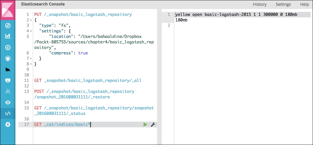
Restoring the data from Console
The response indicates that our index has been created and contains 300,000 documents.
There could be different approaches here to what index topology we should use: because the data has timestamps, we could, for example, create daily indices, or weekly indices. This is very common in a production environment, as the most recent data is often the most used. Thus, from an operations point of view, if the last seven days of logs are the most important ones and you have daily indices, it's very handy to set up routines that either archive or remove the old indices (older than seven days).
If we look at the content of our index, here is an example of a document extract:
"@timestamp": "2015-03-11T21:24:20.000Z",
"host": "Astaire.local",
"clientip": "186.231.123.210",
"ident": "-",
"auth": "-",
"timestamp": "11/Mar/2015:21:24:20 +0000",
"verb": "GET",
"request": "/presentations/logstash-scale11x/lib/js/head.min.js",
"httpversion": "1.1",
"response": 200,
"bytes": 3170,
"referrer": ""http://semicomplete.com/presentations/logstash-scale11x/"",
"agent": ""Mozilla/5.0 (Macintosh; Intel Mac OS X 10_9_0) AppleWebKit/537.36 (KHTML, like Gecko) Chrome/32.0.1700.102 Safari/537.36"",
"geoip": {
  "ip": "186.231.123.210",
  "country_code2": "BR",
  "country_code3": "BRA",
  "country_name": "Brazil",
  "continent_code": "SA",
  "latitude": -10,
  "longitude": -55,
  "location": [
    -55,
    -10
  ]
},
"useragent": {
  "name": "Chrome",
  "os": "Mac OS X 10.9.0",
  "os_name": "Mac OS X",
  "os_major": "10",
  "os_minor": "9",
  "device": "Other",
  "major": "32",
  "minor": "0",
  "patch": "1700"
}
The document describes a given user connection to the website and is composed of HTTP metadata, such as the version, the return code, the verb, the user agent with the description of the OS and device used, and even localization information.
Analyzing each document would not make it possible to understand website-user behavior; this is where Kibana comes into play, by allowing us to create visualizations that will aggregate data and reveal insights.
We can now import the dashboard.
Unlike in the previous chapter, we won't create the visualization here, but rather use the Import feature of Kibana, which lets you import Kibana objects such as searches, visualizations, and dashboards that already exist. All these objects are actually JSON objects indexed in a specific index called, by default, .kibana.
Go into the management section of Kibana and click on Saved Objects. From there, you can click on the Import button and choose the JSON file provided in the book's resources. First import the Apache-logs-visualizations.json file, and then the Apache-logs-dashboard.json file. The first contains all the visualizations, and the second contains the dashboard that uses the visualizations. The following visualizations should be present:
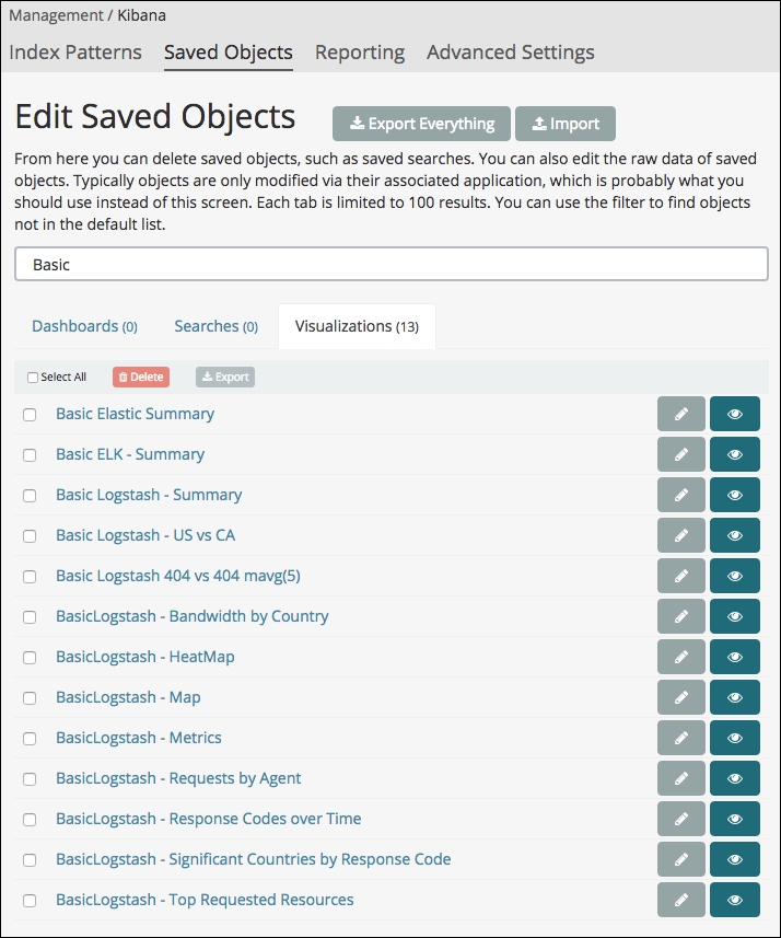
Imported Visualizations
You will have all the BasicLogstash visualizations.
Let's review the imported dashboard. Go to the Dashboard section and try to open the Elastic Stack-Apache Logs dashboard. You should get the following:
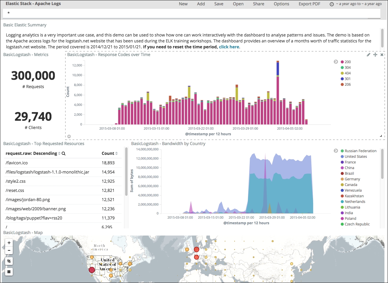
Apache log dashboard
At this stage, we are now ready to browse the visualizations one by one and explain what they mean.
We'll now go through each visualization and look at the key performance indicators and features they provide:
The following is the screenshot of the basic Elastic summary:
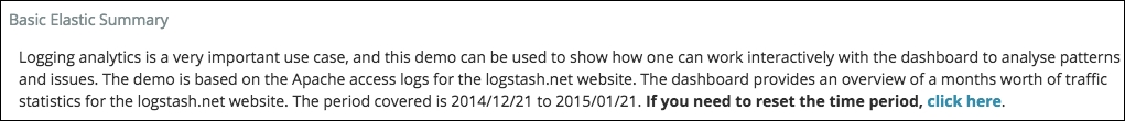
Markdown visualization
The markdown visualization can be used to add comments to your dashboard, such as in our example, to explain what the dashboard is about. You can also leverage the support of URLs to create a menu, so the user is able to switch from one state of the dashboard to another.
The following metrics visualization gives a summary about the data presented in the dashboard:
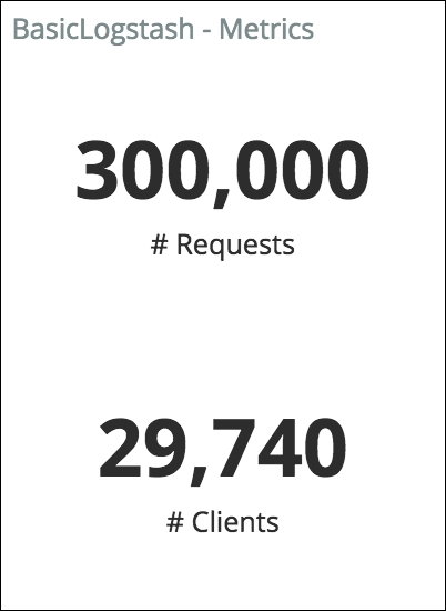
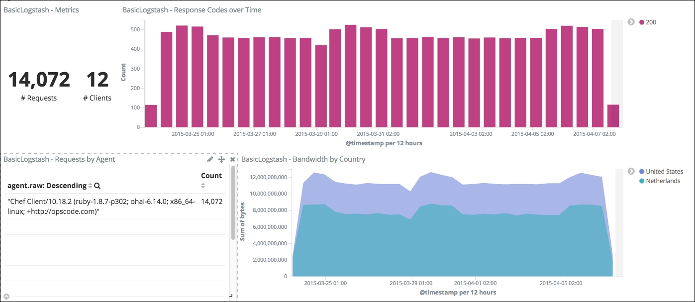
Apache logs metrics
It's always useful to have some metrics displayed in your dashboard, so, for example, you can keep track of the number of documents affected by your filtering while you play with the dashboard.
Bar charts are great for visualizing one or more dimensions of your data over time. In this example, we are showing a breakdown of response code over time. Thus, you can see the volume of requests on www.logstash.net and whether there is a change compared to what you think is the expected behavior. The following shows some 404 spikes that might need a closer look:
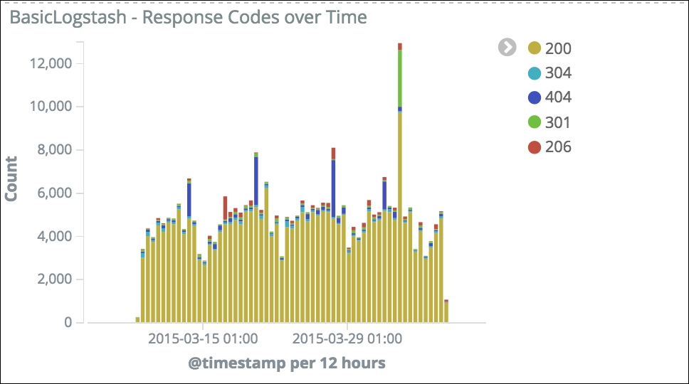
Response codes over time
Area charts are useful for displaying accumulative data over time. Here, we are using the country location field to build this area chart, to give us insights on which countries are connecting to our website:
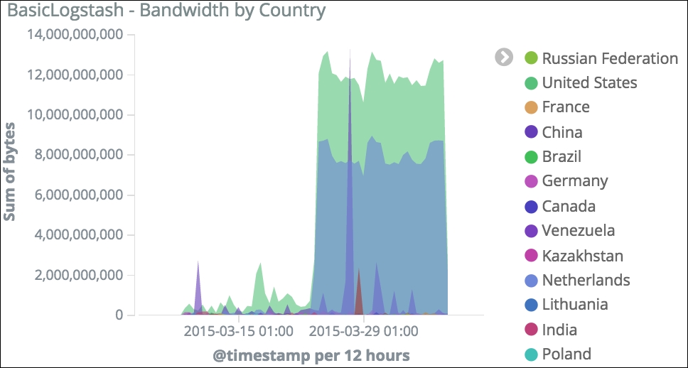
Bandwidth by country
We will look at how we can use this information in the context of bandwidth analysis later in the chapter.
Data table charts can be used to display tabular field information and values. Here, we are displaying a count of the user-agent field, which allows us to understand the types of clients connecting:
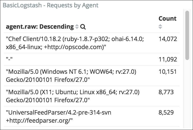
Requests by agent
We will see that in the context of security analytics, this can be a very useful piece of information to identify a security anomaly.
When a host connects to your website, you might to know what to what is the resource is browsing for different reason such as click-stream analysis, or security wise; this is what the following data table gives you:
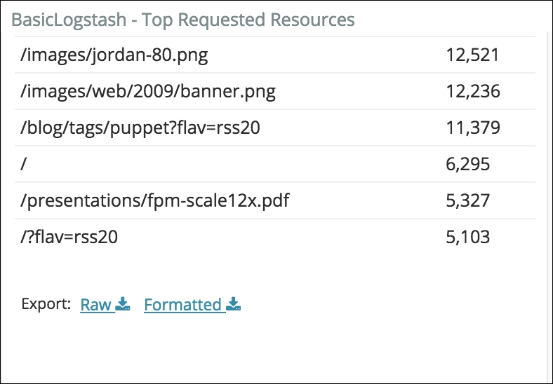
Top requested resources
This is also an asset that we'll use in the security analysis.
The response bar chart already represents two dimensions, where a dimension here is a field contained in our document. We could eventually split by country, but the analysis experience would be a little bit complicated. Instead, we could use a pie chart to show the country breakdown based on the response code, as shown here:
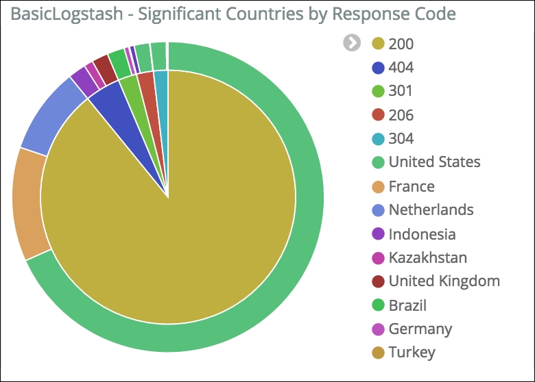
Significant countries by response code
The data contains host geo-point coordinates. Here, we are using this information to graph client connections onto a tile map of the world. Again, from a pure analytics point of view, the fact that countries are mentioned across visualizations wouldn't be enough if they were not drawn on the map as follows:
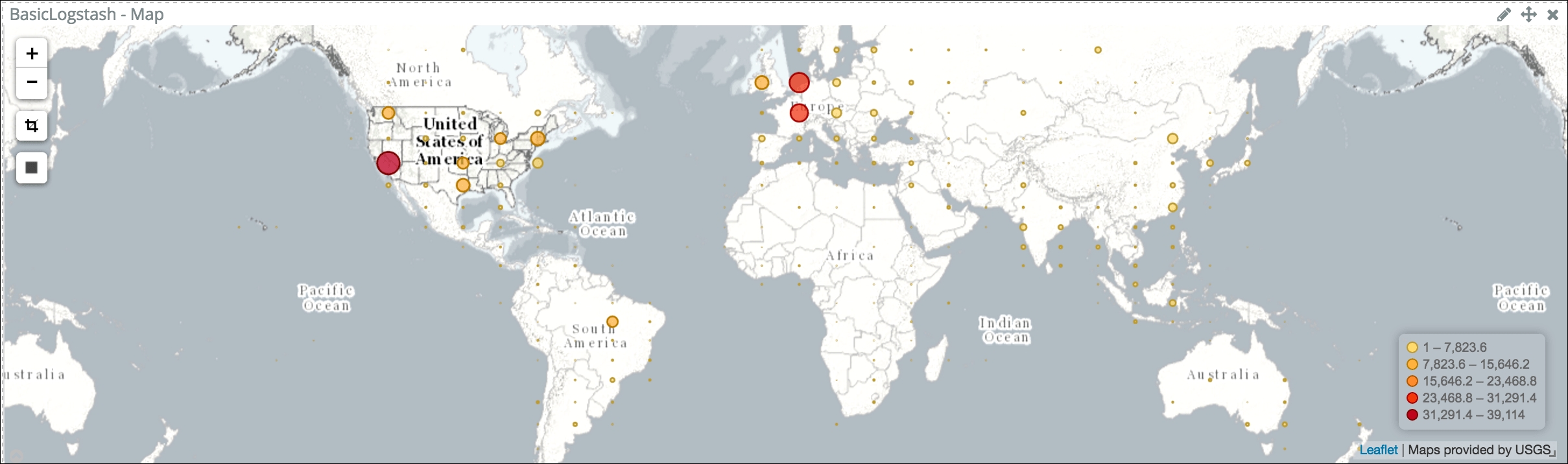
Hits per countries
Furthermore, the map visualization will allow you to draw polygons to narrow down your analysis.
Once the dashboard is created, the idea is to ask it questions by interacting with one or more visualizations. This will narrow down the analysis and isolate the particular patterns that are the answers to our questions.
You may have noticed in the bandwidth by country that the level is low between August 2015 and the end of March 2015 and then suddenly, for an unknown reason, it increases significantly. We see a marked increase in the data downloaded, represented by the arrow on the graph:
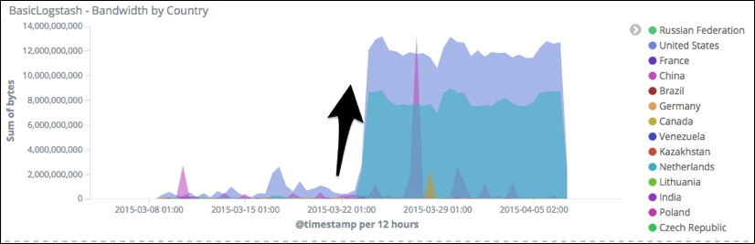
Bandwidth increase
We can zoom into this time region of the chart, which will also zoom in all other charts to within the same time range. If you read the requests by the agent data table, you will notice that the first user agent is a Chef agent. Chef is used by operations teams to automate processes such as installation, for example. Since the data we have comes from www.logstash.net, we can deduce that a Chef agent is connecting to our website for installation purposes.
If you click on the Chef row in the data table, this will apply a dashboard filter based on the value of the field you selected. This allows you to drill into your data, narrowing down your analysis, and we can easily conclude that this process consumes the majority of the bandwidth:
Chef bandwidth utilization
With a few clicks, we have been able to point out a bandwidth utilization issue and are now able to take the proper measures to throttle the connection of such agents to our website. From there, we will switch to a different angle of analysis: security.
In this section, we'll try to look for a security anomaly, which is defined as an unexpected behavior in the data; in other words, data points that are different from normal behavior observed in the data, based on the facts that our dashboard shows us.
If you reset the dashboard by reopening it, you will notice in the bar chart that a significant amount of 404 responses happen sporadically in the background of the hits:
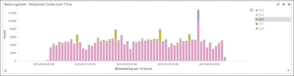
404 responses
Click on the 404 code in the legend to filter the dashboard and refresh the other visualizations and data table. You will notice in the user-agent data table that an agent called - is the source of a lot of the 404 responses. So, let's filter the analysis by clicking on it. Now have a look to the top requested resources:
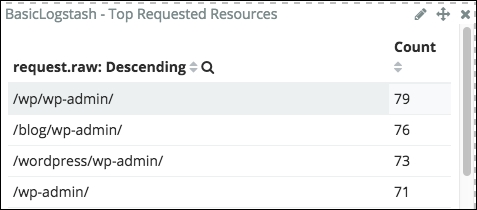
Top requested resources by user agent "-"
There is a very unusual, possibly suspicious activity, such as an attempt to attack our website. Basically, the wp-admin URI is the resource to access the WordPress blog admin console. However, in our case, the website is not a WordPress blog.
New WordPress users may not have the knowledge to either change or disable the admin console on their site, and might also use the default user/password. So, my guess here is that the user agent tried to connect to the wp-admin resource and issue the default credentials to take total control of our website.