Chapter 17. Advanced Function Topics
This chapter introduces a collection of more advanced function-related topics: the lambda expression, functional programming tools such as map and list comprehensions, generator functions and expressions, and more. Part of the art of using functions lies in the interfaces between them, so we will also explore some general function design principles here. Because this is the last chapter in Part IV, we’ll close with the usual sets of gotchas and exercises to help you start coding the ideas you’ve read about.
Anonymous Functions: lambda
You’ve seen what it takes to write your own basic functions in Python. The next sections deal with a few more advanced function-related ideas. Most of these are optional features, but they can simplify your coding tasks when used well.
Besides the def statement, Python also provides an expression form that generates function objects. Because of its similarity to a tool in the LISP language, it’s called lambda.[40] Like def, this expression creates a function to be called later, but it returns the function instead of assigning it to a name. This is why lambdas are sometimes known as anonymous (i.e., unnamed) functions. In practice, they are often used as a way to inline a function definition, or to defer execution of a piece of code.
lambda Expressions
The lambda’s general form is the keyword lambda, followed by one or more arguments (exactly like the arguments list you enclose in parentheses in a def header), followed by an expression after a colon:
lambda
argument1,argument2,...argumentN:expression using arguments
Function objects returned by running lambda expressions work exactly the same as those created and assigned by def, but there are a few differences that make lambdas useful in specialized roles:
lambdais an expression, not a statement. Because of this, alambdacan appear in places adefis not allowed by Python’s syntax—inside a list literal, or function call, for example. Also, as an expression,lambdareturns a value (a new function) that can optionally be assigned a name; in contrast, thedefstatement always assigns the new function to the name in the header, instead of returning it as a result.lambda’s body is a single expression, not a block of statements. Thelambda’s body is similar to what you’d put in adefbody’sreturnstatement; you simply type the result as a naked expression, instead of explicitly returning it. Because it is limited to an expression, alambdais less general than adef—you can only squeeze so much logic into alambdabody without using statements such asif. This is by design—it limits program nesting:lambdais designed for coding simple functions, anddefhandles larger tasks.
Apart from those distinctions, defs and lambdas do the same sort of work. For instance, we’ve seen how to make a function with a def statement:
def func(x, y, z): return x + y + z... >>>func(2, 3, 4)9
But, you can achieve the same effect with a lambda expression by explicitly assigning its result to a name through which you can later call the function:
f = lambda x, y, z: x + y + z>>>f(2, 3, 4)9
Here, f is assigned the function object the lambda expression creates; this is how def works, too, but its assignment is automatic.
Defaults work on lambda arguments, just like in a def:
x = (lambda a="fee", b="fie", c="foe": a + b + c)>>>x("wee")'weefiefoe'
The code in a lambda body also follows the same scope lookup rules as code inside a def. lambda expressions introduce a local scope much like a nested def, which automatically sees names in enclosing functions, the module, and the built-in scope (via the LEGB rule):
def knights( ):...title = 'Sir'...action = (lambda x: title + ' ' + x)# Title in enclosing def ...return action# Return a function ... >>>act = knights( )>>>act('robin')'Sir robin'
In this example, prior to Release 2.2, the value for the name title would typically have been passed in as a default argument value instead; flip back to the scopes coverage in Chapter 16 if you’ve forgotten why.
Why Use lambda?
Generally speaking, lambdas come in handy as a sort of function shorthand that allows you to embed a function’s definition within the code that uses it. They are entirely optional (you can always use defs instead), but they tend to be simpler coding constructs in scenarios where you just need to embed small bits of executable code.
For instance, we’ll see later that callback handlers are frequently coded as inline lambda expressions embedded directly in a registration call’s arguments list, instead of being defined with a def elsewhere in a file, and referenced by name (see the sidebar "Why You Will Care: Callbacks" later in this chapter for an example).
lambdas are also commonly used to code jump tables, which are lists or dictionaries of actions to be performed on demand. For example:
The lambda expression is most useful as a shorthand for def, when you need to stuff small pieces of executable code into places where statements are illegal syntactically. This code snippet, for example, builds up a list of three functions by embedding lambda expressions inside a list literal; a def won’t work inside a list literal like this because it is a statement, not an expression.
You can do the same sort of thing with dictionaries and other data structures in Python to build up action tables:
key = 'got'>>>{'already': (lambda: 2 + 2),...'got': (lambda: 2 * 4),...'one': (lambda: 2 ** 6)...}[key]( )8
Here, when Python makes the dictionary, each of the nested lambdas generates and leaves behind a function to be called later; indexing by key fetches one of those functions, and parentheses force the fetched function to be called. When coded this way, a dictionary becomes a more general multiway branching tool than what I could show you in Chapter 12’s coverage of if statements.
To make this work without lambda, you’d need to instead code three def statements somewhere else in your file, outside the dictionary in which the functions are to be used:
This works, too, but your defs may be arbitrarily far away in your file, even if they are just little bits of code. The code proximity that lambdas provide is especially useful for functions that will only be used in a single context—if the three functions here are not useful anywhere else, it makes sense to embed their definitions within the dictionary as lambdas. Moreover, the def form requires you to make up names for these little functions that may clash with other names in this file.
lambdas also come in handy in function argument lists as a way to inline temporary function definitions not used anywhere else in your program; we’ll see some examples of such other uses later in this chapter, when we study map.
How (Not) to Obfuscate Your Python Code
The fact that the body of a lambda has to be a single expression (not a series of statements) would seem to place severe limits on how much logic you can pack into a lambda. If you know what you’re doing, though, you can code most statements in Python as expression-based equivalents.
For example, if you want to print from the body of a lambda function, simply say sys.stdout.write(str(x)+'
'), instead of print x (recall from Chapter 11 that this is what print really does). Similarly, to nest logic in a lambda, you can use the if/else ternary expression introduced in Chapter 13, or the equivalent but trickier and/or combination also described there. As you learned earlier, the following statement:
can be emulated by either of these roughly equivalent expressions:
Because expressions like these can be placed inside a lambda, they may be used to implement selection logic within a lambda function:
lower = (lambda x, y: x if x < y else y)>>>lower('bb', 'aa')'aa' >>>lower('aa', 'bb')'aa'
Furthermore, if you need to perform loops within a lambda, you can also embed things like map calls and list comprehension expressions (tools we met earlier, in Chapter 13, and will revisit later in this chapter):
import sys>>>showall = (lambda x: map(sys.stdout.write, x))>>>t = showall(['spam ', 'toast ', 'eggs '])spam toast eggs >>>showall = lambda x: [sys.stdout.write(line) for line in x]>>>t = showall(('bright ', 'side ', 'of ', 'life '))bright side of life
Now that I’ve shown you these tricks, I am required by law to ask you to please only use them as a last resort. Without due care, they can lead to unreadable (a.k.a. obfuscated) Python code. In general, simple is better than complex, explicit is better than implicit, and full statements are better than arcane expressions. On the other hand, you may find these techniques useful in moderation.
Nested lambdas and Scopes
lambdas are the main beneficiaries of nested function scope lookup (the E in the LEGB rule we met in Chapter 16). In the following, for example, the lambda appears inside a def—the typical case—and so can access the value that the name x had in the enclosing function’s scope at the time that the enclosing function was called:
def action(x):...return (lambda y: x + y)# Make and return function, remember x ... >>>act = action(99)>>>act<function <lambda> at 0x00A16A88> >>>act(2)101
What wasn’t illustrated in the prior chapter’s discussion of nested function scopes is that a lambda also has access to the names in any enclosing lambda. This case is somewhat obscure, but imagine if we recoded the prior def with a lambda:
action = (lambda x: (lambda y: x + y))>>>act = action(99)>>>act(3)102 >>>((lambda x: (lambda y: x + y))(99))(4)103
Here, the nested lambda structure makes a function that makes a function when called. In both cases, the nested lambda’s code has access to the variable x in the enclosing lambda. This works, but it’s fairly convoluted code; in the interest of readability, nested lambdas are generally best avoided.
Another very common application of lambda is to define inline callback functions for Python’s Tkinter GUI API. For example, the following creates a button that prints a message on the console when pressed:
Here, the callback handler is registered by passing a function generated with a lambda to the command keyword argument. The advantage of lambda over def here is that the code that handles a button press is right here, embedded in the button creation call.
In effect, the lambda defers execution of the handler until the event occurs: the write call happens on button presses, not when the button is created.
Because the nested function scope rules apply to lambdas as well, they are also easier to use as callback handlers, as of Python 2.2—they automatically see names in the functions in which they are coded, and no longer require passed-in defaults in most cases. This is especially handy for accessing the special self instance argument that is a local variable in enclosing class method functions (more on classes in Part VI):
use message...
In prior releases, even self had to be passed in with defaults.
Applying Functions to Arguments
Some programs need to call arbitrary functions in a generic fashion, without knowing their names or arguments ahead of time (we’ll see examples of where this can be useful later). Both the apply built-in function, and some special call syntax available in Python, can do the job.
Tip
At this writing, both apply and the special call syntax described in this section can be used freely in Python 2.5, but it seems likely that apply may go away in Python 3.0. If you wish to future-proof your code, use the equivalent special call syntax, not apply.
The apply Built-in
When you need to be dynamic, you can call a generated function by passing it as an argument to apply, along with a tuple of arguments to pass to that function:
def func(x, y, z): return x + y + z... >>>apply(func, (2, 3, 4))9 >>>f = lambda x, y, z: x + y + z>>>apply(f, (2, 3, 4))9
The apply function simply calls the passed-in function in the first argument, matching the passed-in arguments tuple to the function’s expected arguments. Because the arguments list is passed in as a tuple (i.e., a data structure), a program can build it at runtime.[41]
The real power of apply is that it doesn’t need to know how many arguments a function is being called with. For example, you can use if logic to select from a set of functions and argument lists, and use apply to call any of them:
More generally, apply is useful any time you cannot predict the arguments list ahead of time. If your user selects an arbitrary function via a user interface, for instance, you may be unable to hardcode a function call when writing your script. To work around this, simply build up the arguments list with tuple operations, and call the function indirectly through apply:
args = (2,3) + (4,)>>>args(2, 3, 4) >>>apply(func, args)9
Passing keyword arguments
The apply call also supports an optional third argument, where you can pass in a dictionary that represents keyword arguments to be passed to the function:
def echo(*args, **kwargs): print args, kwargs... >>>echo(1, 2, a=3, b=4)(1, 2) {'a': 3, 'b': 4}
This allows you to construct both positional and keyword arguments at runtime:
pargs = (1, 2)>>>kargs = {'a':3, 'b':4}>>>apply(echo, pargs, kargs)(1, 2) {'a': 3, 'b': 4}
apply-Like Call Syntax
Python also allows you to accomplish the same effect as an apply call with special syntax in the call. This syntax mirrors the arbitrary arguments syntax in def headers that we met in Chapter 16. For example, assuming the names in this example are still as assigned earlier:
apply(func, args)# Traditional: tuple 9 >>>func(*args)# New apply-like syntax 9 >>>echo(*pargs, **kargs)# Keyword dictionaries too (1, 2) {'a': 3, 'b': 4}
This special call syntax is newer than the apply function, and is generally preferred today. It doesn’t have any obvious advantages over an explicit apply call, apart from its symmetry with def headers, and requiring a few less keystrokes. However, the new call syntax alternative also allows us to pass along real additional arguments, and so is more general:
echo(0, *pargs, **kargs)# Normal, *tuple, **dictionary (0, 1, 2) {'a': 3, 'b': 4}
Mapping Functions over Sequences: map
One of the more common things programs do with lists and other sequences is apply an operation to each item and collect the results. For instance, updating all the counters in a list can be done easily with a for loop:
counters = [1, 2, 3, 4]>>> >>>updated = []>>>for x in counters:...updated.append(x + 10)# Add 10 to each item ... >>>updated[11, 12, 13, 14]
But because this is such a common operation, Python actually provides a built-in that does most of the work for you. The map function applies a passed-in function to each item in a sequence object, and returns a list containing all the function call results. For example:
def inc(x): return x + 10# Function to be run ... >>>map(inc, counters)# Collect results [11, 12, 13, 14]
map was introduced as a parallel loop-traversal tool in Chapter 13. As you may recall, we passed in None for the function argument to pair up items. Here, we make better use of it by passing in a real function to be applied to each item in the list—map calls inc on each list item, and collects all the return values into a list.
Because map expects a function to be passed in, it also happens to be one of the places where lambdas commonly appear:
map((lambda x: x + 3), counters)# Function expression [4, 5, 6, 7]
Here, the function adds 3 to each item in the counters list; as this function isn’t needed elsewhere, it was written inline as a lambda. Because such uses of map are equivalent to for loops, with a little extra code, you can always code a general mapping utility yourself:
def mymap(func, seq):...res = []...for x in seq: res.append(func(x))...return res... >>>map(inc, [1, 2, 3])[11, 12, 13] >>>mymap(inc, [1, 2, 3])[11, 12, 13]
However, as map is a built-in, it’s always available, always works the same way, and has some performance benefits (in short, it’s faster than a manually coded for loop). Moreover, map can be used in more advanced ways than shown here. For instance, given multiple sequence arguments, it sends items taken from sequences in parallel as distinct arguments to the function:
pow(3, 4)81 >>>map(pow, [1, 2, 3], [2, 3, 4])# 1**2, 2**3, 3**4 [1, 8, 81]
Here, the pow function takes two arguments on each call—one from each sequence passed to map. Although we could simulate this generality, too, there is no obvious point in doing so when a speedy built-in is provided.
Tip
The map call is similar to the list comprehension expressions we studied in Chapter 13, and will meet again later in this chapter, but map applies a function call to each item instead of an arbitrary expression. Because of this limitation, it is a somewhat less general tool. However, in some cases, map is currently faster to run than a list comprehension (e.g., when mapping a built-in function), and it may require less coding. Because of that, it seems likely that map will still be available in Python 3.0. However, a recent Python 3.0 document did propose removing this call, along with the reduce and filter calls discussed in the next section, from the built-in namespace (they may show up in modules instead).
While map may stick around, it’s likely that reduce and filter will be removed in 3.0, partly because they are redundant with list comprehensions (filter is subsumed by list comprehension if clauses), and partly because of their complexity (reduce is one of the most complex tools in the language and is not intuitive). I cannot predict the future on this issue, though, so be sure to watch the Python 3.0 release notes for more on these possible changes. These tools are all still included in this edition of the book because they are part of the current version of Python, and will likely be present in Python code you’re likely to see for some time to come.
Functional Programming Tools: filter and reduce
The map function is the simplest representative of a class of Python built-ins used for functional programming—which mostly just means tools that apply functions to sequences. Its relatives filter out items based on a test function (filter), and apply functions to pairs of items and running results (reduce). For example, the following filter call picks out items in a sequence that are greater than zero:
range(−5, 5)[−5, −4, −3, −2, −1, 0, 1, 2, 3, 4] >>>filter((lambda x: x > 0), range(−5, 5))[1, 2, 3, 4]
Items in the sequence for which the function returns true are added to the result list. Like map, this function is roughly equivalent to a for loop, but is built-in, and fast:
res = [ ]>>>for x in range(−5, 5):...if x > 0:...res.append(x)... >>>res[1, 2, 3, 4]
reduce is more complex. Here are two reduce calls computing the sum and product of items in a list:
reduce((lambda x, y: x + y), [1, 2, 3, 4])10 >>>reduce((lambda x, y: x * y), [1, 2, 3, 4])24
At each step, reduce passes the current sum or product, along with the next item from the list, to the passed-in lambda function. By default, the first item in the sequence initializes the starting value. Here’s the for loop equivalent to the first of these calls, with the addition hardcoded inside the loop:
L = [1,2,3,4]>>>res = L[0]>>>for x in L[1:]:...res = res + x... >>> res 10
Coding your own version of reduce (for instance, if it is indeed removed in Python 3.0) is actually fairly straightforward:
def myreduce(function, sequence):...tally = sequence[0]...for next in sequence[1:]:...tally = function(tally, next)...return tally... >>>myreduce((lambda x, y: x + y), [1, 2, 3, 4, 5])15 >>>myreduce((lambda x, y: x * y), [1, 2, 3, 4, 5])120
If this has sparked your interest, also see the built-in operator module, which provides functions that correspond to built-in expressions, and so comes in handy for some uses of functional tools:
import operator>>>reduce(operator.add, [2, 4, 6])# Function-based + 12 >>>reduce((lambda x, y: x + y), [2, 4, 6])12
Together with map, filter and reduce support powerful functional programming techniques. Some observers might also extend the functional programming toolset in Python to include lambda and apply, and list comprehensions, which are discussed in the next section.
List Comprehensions Revisited: Mappings
Because mapping operations over sequences and collecting results is such a common task in Python coding, Python 2.0 sprouted a new feature—the list comprehension expression—that makes it even simpler than using the tools we just studied. We met list comprehensions in Chapter 13, but because they’re related to functional programming tools like the map and filter calls, we’ll resurrect the topic here for one last look. Technically, this feature is not tied to functions—as we’ll see, list comprehensions can be a more general tool than map and filter—but it is sometimes best understood by analogy to function-based alternatives.
List Comprehension Basics
Let’s work through an example that demonstrates the basics. As we saw in Chapter 7, Python’s built-in ord function returns the ASCII integer code of a single character (the chr built-in is the converse—it returns the character for an ASCII integer code):
ord('s')115
Now, suppose we wish to collect the ASCII codes of all characters in an entire string. Perhaps the most straightforward approach is to use a simple for loop, and append the results to a list:
res = []>>>for x in 'spam': ...res.append(ord(x))... >>>res[115, 112, 97, 109]
Now that we know about map, though, we can achieve similar results with a single function call without having to manage list construction in the code:
res = map(ord, 'spam')# Apply function to sequence >>>res[115, 112, 97, 109]
As of Python 2.0, however, we can get the same results from a list comprehension expression:
res = [ord(x) for x in 'spam']# Apply expression to sequence >>>res[115, 112, 97, 109]
List comprehensions collect the results of applying an arbitrary expression to a sequence of values and return them in a new list. Syntactically, list comprehensions are enclosed in square brackets (to remind you that they construct lists). In their simple form, within the brackets you code an expression that names a variable followed by what looks like a for loop header that names the same variable. Python then collects the expression’s results for each iteration of the implied loop.
The effect of the preceding example is similar to that of the manual for loop and the map call. List comprehensions become more convenient, though, when we wish to apply an arbitrary expression to a sequence:
[x ** 2 for x in range(10)][0, 1, 4, 9, 16, 25, 36, 49, 64, 81]
Here, we’ve collected the squares of the numbers 0 through 9 (we’re just letting the interactive prompt print the resulting list; assign it to a variable if you need to retain it). To do similar work with a map call, we would probably invent a little function to implement the square operation. Because we won’t need this function elsewhere, we’d typically (but not necessarily) code it inline, with a lambda, instead of using a def statement elsewhere:
map((lambda x: x ** 2), range(10))[0, 1, 4, 9, 16, 25, 36, 49, 64, 81]
This does the same job, and it’s only a few keystrokes longer than the equivalent list comprehension. It’s also only marginally more complex (at least, once you understand the lambda). For more advanced kinds of expressions, though, list comprehensions will often require considerably less typing. The next section shows why.
Adding Tests and Nested Loops
List comprehensions are even more general than shown so far. For instance, you can code an if clause after the for, to add selection logic. List comprehensions with if clauses can be thought of as analogous to the filter built-in discussed in the prior section—they skip sequence items for which the if clause is not true. Here are examples of both schemes picking up even numbers from 0 to 4; like the map list comprehension alternative we just looked at, the filter version here invents a little lambda function for the test expression. For comparison, the equivalent for loop is shown here as well:
[x for x in range(5) if x % 2 == 0][0, 2, 4] >>>filter((lambda x: x % 2 == 0), range(5))[0, 2, 4] >>>res = [ ]>>>for x in range(5):...if x % 2 == 0:...res.append(x)... >>>res[0, 2, 4]
All of these use the modulus (remainder of division) operator, %, to detect even numbers: if there is no remainder after dividing a number by two, it must be even. The filter call is not much longer than the list comprehension here either. However, we can combine an if clause, and an arbitrary expression in our list comprehension, to give it the effect of a filter and a map, in a single expression:
[x ** 2 for x in range(10) if x % 2 == 0][0, 4, 16, 36, 64]
This time, we collect the squares of the even numbers from 0 through 9: the for loop skips numbers for which the attached if clause on the right is false, and the expression on the left computes the squares. The equivalent map call would require a lot more work on our part—we would have to combine filter selections with map iteration, making for a noticeably more complex expression:
map((lambda x: x**2), filter((lambda x: x % 2 == 0), range(10)))[0, 4, 16, 36, 64]
In fact, list comprehensions are more general still. You can code any number of nested for loops in a list comprehension, and each may have an optional associated if test. The general structure of list comprehensions looks like this:
target1insequence1[ifcondition] fortarget2insequence2[ifcondition] ... fortargetNinsequenceN[ifcondition] ]
When for clauses are nested within a list comprehension, they work like equivalent nested for loop statements. For example, the following:
res = [x + y for x in [0, 1, 2] for y in [100, 200, 300]]>>>res[100, 200, 300, 101, 201, 301, 102, 202, 302]
has the same effect as this substantially more verbose equivalent:
res = []>>>for x in [0, 1, 2]:...for y in [100, 200, 300]:...res.append(x + y)... >>>res[100, 200, 300, 101, 201, 301, 102, 202, 302]
Although list comprehensions construct lists, remember that they can iterate over any sequence or other iterable type. Here’s a similar bit of code that traverses strings instead of lists of numbers, and so collects concatenation results:
[x + y for x in 'spam' for y in 'SPAM']['sS', 'sP', 'sA', 'sM', 'pS', 'pP', 'pA', 'pM', 'aS', 'aP', 'aA', 'aM', 'mS', 'mP', 'mA', 'mM']
Finally, here is a much more complex list comprehension that illustrates the effect of attached if selections on nested for clauses:
[(x, y) for x in range(5) if x % 2 == 0 for y in range(5) if y % 2 == 1][(0, 1), (0, 3), (2, 1), (2, 3), (4, 1), (4, 3)]
This expression permutes even numbers from 0 through 4 with odd numbers from 0 through 4. The if clauses filter out items in each sequence iteration. Here’s the equivalent statement-based code:
res = []>>>for x in range(5):...if x % 2 == 0:...for y in range(5):...if y % 2 == 1:...res.append((x, y))... >>>res[(0, 1), (0, 3), (2, 1), (2, 3), (4, 1), (4, 3)]
Recall that if you’re confused about what a complex list comprehension does, you can always nest the list comprehension’s for and if clauses inside each other (indenting successively further to the right) to derive the equivalent statements. The result is longer, but perhaps clearer.
The map and filter equivalent would be wildly complex and deeply nested, so I won’t even try showing it here. I’ll leave its coding as an exercise for Zen masters, ex-LISP programmers, and the criminally insane.
List Comprehensions and Matrixes
Let’s look at one more advanced application of list comprehensions to stretch a few synapses. One basic way to code matrixes (a.k.a. multidimensional arrays) in Python is with nested list structures. The following, for example, defines two 3 × 3 matrixes as lists of nested lists:
M = [[1, 2, 3],...[4, 5, 6],...[7, 8, 9]]>>>N = [[2, 2, 2],...[3, 3, 3],...[4, 4, 4]]
Given this structure, we can always index rows, and columns within rows, using normal index operations:
M[1] [4, 5, 6]>>>M[1][2]6
List comprehensions are powerful tools for processing such structures, though, because they automatically scan rows and columns for us. For instance, although this structure stores the matrix by rows, to collect the second column, we can simply iterate across the rows and pull out the desired column, or iterate through positions in the rows and index as we go:
[row[1] for row in M][2, 5, 8] >>>[M[row][1] for row in (0, 1, 2)][2, 5, 8]
Given positions, we can also easily perform tasks such as pulling out a diagonal. The following expression uses range to generate the list of offsets, and then indexes with the row and column the same, picking out M[0][0], then M[1][1], and so on (we assume the matrix has the same number of rows and columns):
[M[i][i] for i in range(len(M))][1, 5, 9]
Finally, with a bit of creativity, we can also use list comprehensions to combine multiple matrixes. The following first builds a flat list that contains the result of multiplying the matrixes pairwise, and then builds a nested list structure having the same values by nesting list comprehensions:
[M[row][col] * N[row][col] for row in range(3) for col in range(3)][2, 4, 6, 12, 15, 18, 28, 32, 36] >>>[[M[row][col] * N[row][col] for col in range(3)] for row in range(3)][[2, 4, 6], [12, 15, 18], [28, 32, 36]]
This last expression works because the row iteration is an outer loop: for each row, it runs the nested column iteration to build up one row of the result matrix. It’s equivalent to this statement-based code:
res = []>>>for row in range(3):...tmp = []...for col in range(3):...tmp.append(M[row][col] * N[row][col])...res.append(tmp)... >>>res[[2, 4, 6], [12, 15, 18], [28, 32, 36]]
Compared to these statements, the list comprehension version requires only one line of code, will probably run substantially faster for large matrixes, and just might make your head explode! Which brings us to the next section.
Comprehending List Comprehensions
With such generality, list comprehensions can quickly become, well, incomprehensible, especially when nested. Consequently, my advice is typically to use simple for loops when getting started with Python, and map calls in most other cases (unless they get too complex). The “keep it simple” rule applies here, as always: code conciseness is a much less important goal than code readability.
However, in this case, there is currently a substantial performance advantage to the extra complexity: based on tests run under Python today, map calls are roughly twice as fast as equivalent for loops, and list comprehensions are usually slightly faster than map calls.[42] This speed difference is down to the fact that map and list comprehensions run at C language speed inside the interpreter, which is much faster than stepping through Python for loop code within the PVM.
Because for loops make logic more explicit, I recommend them in general on the grounds of simplicity. However, map and list comprehensions are worth knowing and using for simpler kinds of iterations, and if your application’s speed is an important consideration. In addition, because map and list comprehensions are both expressions, they can show up syntactically in places that for loop statements cannot, such as in the bodies of lambda functions, within list and dictionary literals, and more. Still, you should try to keep your map calls and list comprehensions simple; for more complex tasks, use full statements instead.
Here’s a more realistic example of list comprehensions and map in action (we solved this problem with list comprehensions in Chapter 13, but we’ll revive it here to add map-based alternatives). Recall that the file readlines method returns lines with
end-of-line characters at the ends:
open('myfile').readlines( )['aaa ', 'bbb ', 'ccc ']
If you don’t want the end-of-line characters, you can slice them off all the lines in a single step with a list comprehension or a map call:
[line.rstrip( ) for line in open('myfile').readlines( )]['aaa', 'bbb', 'ccc'] >>>[line.rstrip( ) for line in open('myfile')]['aaa', 'bbb', 'ccc'] >>>map((lambda line: line.rstrip( )), open('myfile'))['aaa', 'bbb', 'ccc']
The last two of these make use of file iterators (which essentially means that you don’t need a method call to grab all the lines in iteration contexts such as these). The map call is just slightly longer than the list comprehension, but neither has to manage result list construction explicitly.
A list comprehension can also be used as a sort of column projection operation. Python’s standard SQL database API returns query results as a list of tuples much like the following—the list is the table, tuples are rows, and items in tuples are column values:
A for loop could pick up all the values from a selected column manually, but map and list comprehensions can do it in a single step, and faster:
[age for (name, age, job) in listoftuple][35, 40] >>>map((lambda (name, age, job): age), listoftuple)[35, 40]
Both of these make use of tuple assignment to unpack row tuples in the list.
See other books and resources for more on Python’s database API.
Iterators Revisited: Generators
In this part of the book, we’ve learned about coding normal functions that receive input parameters and send back a single result immediately. It is also possible, however, to write functions that may send back a value and later be resumed, picking up where they left off. Such functions are known as generators because they generate a sequence of values over time.
Generator functions are like normal functions in most respects, but in Python, they are automatically made to implement the iteration protocol so that they can appear in iteration contexts. We studied iterators in Chapter 13; here, we’ll revise them to see how they relate to generators.
Unlike normal functions that return a value and exit, generator functions automatically suspend and resume their execution and state around the point of value generation. Because of that, they are often a useful alternative to both computing an entire series of values up front, and manually saving and restoring state in classes. Generator functions automatically retain their state when they are suspended—because this includes their entire local scope, their local variables keep state information, which is available when the functions are resumed.
The chief code difference between generator and normal functions is that a generator yields a value, rather than returning one—the yield statement suspends the function, and sends a value back to the caller, but retains enough state to enable the function to resume from where it left off. This allows these functions to produce a series of values over time, rather than computing them all at once, and sending them back in something like a list.
Generator functions are bound up with the notion of iterator protocols in Python. In short, functions containing a yield statement are compiled specially as generators; when called, they return a generator object that supports the iterator object interface. Generator functions may also have a return statement, which simply terminates the generation of values.
Iterator objects, in turn, define a next method, which either returns the next item in the iteration, or raises a special exception (StopIteration) to end the iteration. Iterators are fetched with the iter built-in function. Python for loops use this iteration interface protocol to step through a sequence (or sequence generator), if the protocol is supported; if not, for falls back on repeatedly indexing sequences instead.
Generator Function Example
Generators and iterators are advanced language features, so please see the Python library manuals for the full story. To illustrate the basics, though, the following code defines a generator function that can be used to generate the squares of a series of numbers over time:[43]
def gensquares(N):...for i in range(N):...yield i ** 2# Resume here later ...
This function yields a value, and so returns to its caller, each time through the loop; when it is resumed, its prior state is restored, and control picks up again immediately after the yield statement. For example, when used in the body of a for loop, control returns to the function after its yield statement each time through the loop:
for i in gensquares(5):# Resume the function ...print i, ':',# Print last yielded value ... 0 : 1 : 4 : 9 : 16 : >>>
To end the generation of values, functions either use a return statement with no value, or simply allow control to fall off the end of the function body.
If you want to see what is going on inside the for, call the generator function directly:
x = gensquares(4)>>>x<generator object at 0x0086C378>
You get back a generator object that supports the iterator protocol (i.e., has a next method that starts the function, or resumes it from where it last yielded a value, and raises a StopIteration exception when the end of the series of values is reached):
x.next( )0 >>>x.next( )1 >>>x.next( )4 >>>x.next( )9 >>>x.next( )Traceback (most recent call last): File "<pyshell#453>", line 1, in <module> x.next( ) StopIteration
for loops work with generators in the same way—by calling the next method repeatedly, until an exception is caught. If the object to be iterated over does not support this protocol, for loops instead use the indexing protocol to iterate.
Note that in this example, we could also simply build the list of yielded values all at once:
def buildsquares(n):...res = []...for i in range(n): res.append(i**2)...return res... >>>for x in buildsquares(5): print x, ':',... 0 : 1 : 4 : 9 : 16 :
For that matter, we could use any of the for loop, map, or list comprehension techniques:
for x in [n**2 for n in range(5)]:...print x, ':', ... 0 : 1 : 4 : 9 : 16 : >>>for x in map((lambda x:x**2), range(5)):...print x, ':',... 0 : 1 : 4 : 9 : 16 :
However, generators allow functions to avoid doing all the work up front, which is especially useful when the result lists are large, or when it takes a lot of computation to produce each value. Generators distribute the time required to produce the series of values among loop iterations. Moreover, for more advanced uses, they provide a simpler alternative to manually saving the state between iterations in class objects (more on classes later in Part VI); with generators, function variables are saved and restored automatically.
Extended Generator Function Protocol: send Versus next
In Python 2.5, a send method was added to the generator function protocol. The send method advances to the next item in the series of results, just like the next method, but also provides a way for the caller to communicate with the generator, to affect its operation.
Technically, yield is now an expression form that returns the item passed to send, not a statement (though it can be called either way—as yield X, or A = (yield X)). Values are sent into a generator by calling its send(value) method. The generator’s code is then resumed, and the yield expression returns the value passed to send. If the regular next( ) method is called, the yield returns None.
The send method can be used, for example, to code a generator that can be terminated by its caller. In addition, generators in 2.5 also support a throw(type) method to raise an exception inside the generator at the latest yield, and a close( ) method that raises a new GeneratorExit exception inside the generator to terminate the iteration. These are advanced features that we won’t delve into in more detail here; see Python’s standard manuals for more details.
Iterators and Built-in Types
As we saw in Chapter 13, built-in data types are designed to produce iterator objects in response to the iter built-in function. Dictionary iterators, for instance, produce key list items on each iteration:
D = {'a':1, 'b':2, 'c':3}>>>x = iter(D)>>>x.next( )'a' >>>x.next( )'c'
In addition, all iteration contexts (including for loops, map calls, list comprehensions, and the many other contexts we met in Chapter 13) are in turn designed to automatically call the iter function to see whether the protocol is supported. That’s why you can loop through a dictionary’s keys without calling its keys method, step through lines in a file without calling readlines or xreadlines, and so on:
for key in D:...print key, D[key]... a 1 c 3 b 2
As we’ve also seen, for file iterators, Python simply loads lines from the file on demand:
for line in open('temp.txt'):...print line,... Tis but a flesh wound.
It is also possible to implement arbitrary generator objects with classes that conform to the iterator protocol, and so may be used in for loops and other iteration contexts. Such classes define a special _ _iter_ _ method that returns an iterator object (preferred over the _ _getitem_ _ indexing method). However, this is well beyond the scope of this chapter; see Part VI for more on classes in general, and Chapter 24 for an example of a class that implements the iterator protocol.
Generator Expressions: Iterators Meet List Comprehensions
In recent versions of Python, the notions of iterators and list comprehensions are combined in a new feature of the language, generator expressions. Syntactically, generator expressions are just like normal list comprehensions, but they are enclosed in parentheses instead of square brackets:
[x ** 2 for x in range(4)]# List comprehension: build a list [0, 1, 4, 9] >>>(x ** 2 for x in range(4))# Generator expression: make an iterable <generator object at 0x011DC648>
Operationally, however, generator expressions are very different—instead of building the result list in memory, they return a generator object, which in turn supports the iteration protocol to yield one piece of the result list at a time in any iteration context:
G = (x ** 2 for x in range(4))>>>G.next( )0 >>>G.next( )1 >>>G.next( )4 >>>G.next( )9 >>>G.next( )Traceback (most recent call last): File "<pyshell#410>", line 1, in <module> G.next( ) StopIteration
We don’t typically see the next iterator machinery under the hood of a generator expression like this because for loops trigger it for us automatically:
for num in (x ** 2 for x in range(4)):...print '%s, %s' % (num, num / 2.0)... 0, 0.0 1, 0.5 4, 2.0 9, 4.5
In fact, every iteration context does this, including the sum, map, and sorted built-in functions, and the other iteration contexts we learned about in Chapter 13, such as the any, all, and list built-in functions.
Notice that the parentheses are not required around a generator expression if they are the sole item enclosed in other parentheses, like those of a function call. Extra parentheses are required, however, in the second call to sorted:
sum(x ** 2 for x in range(4))14 >>>sorted(x ** 2 for x in range(4))[0, 1, 4, 9] >>>sorted((x ** 2 for x in range(4)), reverse=True)[9, 4, 1, 0] >>>import math>>>map(math.sqrt, (x ** 2 for x in range(4)))[0.0, 1.0, 2.0, 3.0]
Generator expressions are primarily a memory space optimization—they do not require the entire result list to be constructed all at once, as the square-bracketed list comprehension does. They may also run slightly slower in practice, so they are probably best used only for very large result sets—which provides a natural segue to the next section.
Timing Iteration Alternatives
We’ve met a few iteration alternatives in this book. To summarize, let’s take a brief look at a case study that pulls together some of the things we’ve learned about iteration and functions.
I’ve mentioned a few times that list comprehensions have a speed performance advantage over for loop statements, and that map performance can be better or worse depending on call patterns. The generator expressions of the prior section tend to be slightly slower than list comprehensions, though they minimize memory requirements.
All that’s true today, but relative performance can vary over time (Python is constantly being optimized). If you want to test this for yourself, try running the following script on your own computer, and your version of Python:
This script tests all the alternative ways to build lists of results and, as shown, executes on the order of 10 million steps for each—that is, each of the four tests builds a list of 10,000 items 1,000 times.
Notice how we have to run the generator expression though the built-in list call to force it to yield all of its values; if we did not, we would just produce a generator that never does any real work. Also, notice how the code at the bottom steps through a tuple of four function objects, and prints the _ _name_ _ of each: this is a built-in attribute that gives a function’s name.
When I ran this in IDLE on Windows XP with Python 2.5, here is what I found—list comprehensions were roughly twice as fast as equivalent for loop statements, and map was slightly quicker than list comprehensions when mapping a built-in function such as abs (absolute value):
But watch what happens if we change this script to perform a real operation on each iteration, such as addition:
The function-call requirement of the map call then makes it just as slow as the for loop statements, despite the fact the looping statements version is larger in terms of code:
Because the interpreter optimizes so much internally, performance analysis of Python code like this is a very tricky affair. It’s virtually impossible to guess which method will perform the best—the best you can do is time your own code, on your computer, with your version of Python. In this case, all we can say for certain is that on this Python, using a user-defined function in map calls can slow it down by at least a factor of 2, and that list comprehensions run quickest for this test.
As I’ve mentioned before, however, performance should not be your primary concern when writing Python code—write for readability and simplicity first, then optimize later, if and only if needed. It could very well be that any of the four alternatives is quick enough for the data sets the program needs to process; if so, program clarity should be the chief goal.
For more insight, try modifying the repetition counts at the top of this script, or see the newer timeit module, which automates timing of code, and finesses some platform-specific issues (on some platforms, for instance, time.time is preferred over time.clock). Also, see the profile standard library module for a complete source code profiler tool.
Function Design Concepts
When you start using functions, you’re faced with choices about how to glue components together—for instance, how to decompose a task into purposeful functions (resulting in cohesion), how your functions should communicate (coupling), and so on. You need to take into account concepts such as cohesion, coupling, and the size of the functions—some of this falls into the category of structured analysis and design. We introduced some ideas related to function and module coupling in the prior chapter, but here is a review of a few general guidelines for Python beginners:
Coupling: use arguments for inputs and
returnfor outputs. Generally, you should strive to make a function independent of things outside of it. Arguments andreturnstatements are often the best ways to isolate external dependencies to a small number of well-known places in your code.Coupling: use global variables only when truly necessary. Global variables (i.e., names in the enclosing module) are usually a poor way for functions to communicate. They can create dependencies and timing issues that make programs difficult to debug and change.
Coupling: don’t change mutable arguments unless the caller expects it. Functions can change parts of passed-in mutable objects, but as with global variables, this implies lots of coupling between the caller and callee, which can make a function too specific and brittle.
Cohesion: each function should have a single, unified purpose. When designed well, each of your functions should do one thing—something you can summarize in a simple declarative sentence. If that sentence is very broad (e.g., “this function implements my whole program”), or contains lots of conjunctions (e.g., “this function gives employee raises and submits a pizza order”), you might want to think about splitting it into separate and simpler functions. Otherwise, there is no way to reuse the code behind the steps mixed together in the function.
Size: each function should be relatively small. This naturally follows from the preceding goal, but if your functions start spanning multiple pages on your display, it’s probably time to split them. Especially given that Python code is so concise to begin with, a long or deeply nested function is often a symptom of design problems. Keep it simple, and keep it short.
Coupling: avoid changing variables in another module file directly. We introduced this concept in the prior chapter, and we’ll revisit it in the next part of the book when we focus on modules. For reference, though, remember that changing variables across file boundaries sets up a coupling between modules similar to how global variables couple functions—the modules become difficult to understand and reuse. Use accessor functions whenever possible, instead of direct assignment statements.
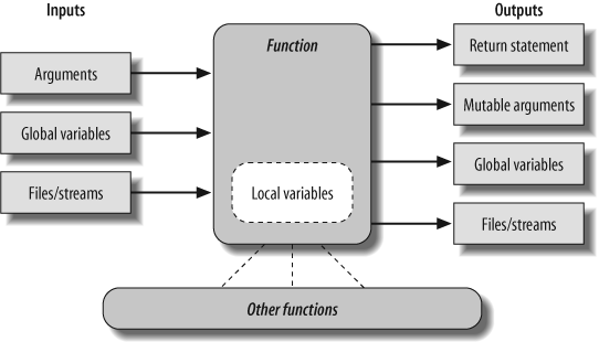
Figure 17-1 summarizes the ways functions can talk to the outside world; inputs may come from items on the left side, and results may be sent out in any of the forms on the right. Many function designers prefer to use only arguments for inputs, and return statements for outputs.
Of course, there are plenty of exceptions to the preceding design rules, including some related to Python’s OOP support. As you’ll see in Part VI, Python classes depend on changing a passed-in mutable object—class functions set attributes of an automatically passed-in argument called self to change per-object state information (e.g., self.name='bob'). Moreover, if classes are not used, global variables are often the best way for functions in modules to retain state between calls. The side effects aren’t dangerous if they’re expected.
Functions Are Objects: Indirect Calls
Because Python functions are objects at runtime, you can write programs that process them generically. Function objects can be assigned, passed to other functions, stored in data structures, and so on, as if they were simple numbers or strings. We’ve seen some of these uses in earlier examples. Function objects also happen to support a special operation: they can be called by listing arguments in parentheses after a function expression. Still, functions belong to the same general category as other objects.
For instance, there’s really nothing special about the name used in a def statement: it’s just a variable assigned in the current scope, as if it had appeared on the left of an = sign. After a def runs, the function name is simply a reference to an object, and you can reassign that object to other names, and call it through any reference (not just the original name):
def echo(message):# echo assigned to a function object ...print message... >>>x = echo# Now x references it too >>>x('Hello world!')# Call the object by adding ( ) Hello world!
Because arguments are passed by assigning objects, it’s just as easy to pass functions to other functions as arguments. The callee may then call the passed-in function just by adding arguments in parentheses:
def indirect(func, arg):...func(arg)# Call the object by adding ( ) ... >>>indirect(echo, 'Hello jello!')# Pass the function to a function Hello jello!
You can even stuff function objects into data structures, as though they were integers or strings. Because Python compound types can contain any sort of object, there’s no special case here either:
schedule = [ (echo, 'Spam!'), (echo, 'Ham!') ]>>>for (func, arg) in schedule:...func(arg)... Spam! Ham!
This code simply steps through the schedule list, calling the echo function with one argument each time through (notice the tuple-unpacking assignment in the for loop header, introduced in Chapter 13). Python’s lack of type declarations makes for an incredibly flexible programming language.
Function Gotchas
Functions have some jagged edges that you might not expect. They’re all obscure, and a few have started to fall away from the language completely in recent releases, but most have been known to trip up new users.
Local Names Are Detected Statically
As you know, Python classifies names assigned in a function as locals by default; they live in the function’s scope and exist only while the function is running. What I didn’t tell you is that Python detects locals statically, when it compiles the def’s code, rather than by noticing assignments as they happen at runtime. This leads to one of the most common oddities posted on the Python newsgroup by beginners.
Normally, a name that isn’t assigned in a function is looked up in the enclosing module:
X = 99>>>def selector( ):# X used but not assigned ...print X# X found in global scope ... >>>selector( )99
Here, the X in the function resolves to the X in the module. But watch what happens if you add an assignment to X after the reference:
def selector( ):...print X# Does not yet exist! ...X = 88# X classified as a local name (everywhere) ... # Can also happen if "import X", "def X" . . . >>>selector( )Traceback (most recent call last): File "<stdin>", line 1, in ? File "<stdin>", line 2, in selector UnboundLocalError: local variable 'X' referenced before assignment
You get an undefined name error, but the reason is subtle. Python reads and compiles this code when it’s typed interactively or imported from a module. While compiling, Python sees the assignment to X, and decides that X will be a local name everywhere in the function. But, when the function is actually run, because the assignment hasn’t yet happened when the print executes, Python says you’re using an undefined name. According to its name rules, it should say this; the local X is used before being assigned. In fact, any assignment in a function body makes a name local. Imports, =, nested defs, nested classes, and so on, are all susceptible to this behavior.
The problem occurs because assigned names are treated as locals everywhere in a function, not just after the statements where they are assigned. Really, the previous example is ambiguous at best: was the intention to print the global X and then create a local X, or is this a genuine programming error? Because Python treats X as a local everywhere, it is an error; if you really mean to print the global X, you need to declare it in a global statement:
def selector( ):...global X# Force X to be global (everywhere) ...print X...X = 88... >>>selector( )99
Remember, though, that this means the assignment also changes the global X, not a local X. Within a function, you can’t use both local and global versions of the same simple name. If you really meant to print the global, and then set a local of the same name, import the enclosing module, and use module attribute notation to get to the global version:
X = 99>>>def selector( ):...import _ _main_ _# Import enclosing module ...print _ _main_ _.X# Qualify to get to global version of name ...X = 88# Unqualified X classified as local ...print X# Prints local version of name ... >>>selector( )99 88
Qualification (the .X part) fetches a value from a namespace object. The interactive namespace is a module called _ _main_ _, so _ _main_ _.X reaches the global version of X. If that isn’t clear, check out Part V.[44]
Defaults and Mutable Objects
Default argument values are evaluated and saved when a def statement is run, not when the resulting function is called. Internally, Python saves one object per default argument attached to the function itself.
That’s usually what you want—because defaults are evaluated at def time, it lets you save values from the enclosing scope, if needed. But because a default retains an object between calls, you have to be careful about changing mutable defaults. For instance, the following function uses an empty list as a default value, and then changes it in-place each time the function is called:
def saver(x=[]):# Saves away a list object ...x.append(1)# Changes same object each time! ...print x... >>>saver([2])# Default not used [2, 1] >>>saver( )# Default used [1] >>>saver( )# Grows on each call! [1, 1] >>>saver( )[1, 1, 1]
Some see this behavior as a feature—because mutable default arguments retain their state between function calls, they can serve some of the same roles as static local function variables in the C language. In a sense, they work sort of like global variables, but their names are local to the functions, and so will not clash with names elsewhere in a program.
To most observers, though, this seems like a gotcha, especially the first time they run into it. There are better ways to retain state between calls in Python (e.g., using classes, which will be discussed in Part VI).
Moreover, mutable defaults are tricky to remember (and to understand at all). They depend upon the timing of default object construction. In the prior example, there is just one list object for the default value—the one created when the def is executed. You don’t get a new list every time the function is called, so the list grows with each new append; it is not reset to empty on each call.
If that’s not the behavior you want, simply make a copy of the default at the start of the function body, or move the default value expression into the function body. As long as the value resides in code that’s actually executed each time the function runs, you’ll get a new object each time through:
def saver(x=None):...if x is None:# No argument passed? ...x = []# Run code to make a new list ...x.append(1)# Changes new list object ...print x... >>>saver([2])[2, 1] >>>saver( )# Doesn't grow here [1] >>>saver( )[1]
By the way, the if statement in this example could almost be replaced by the assignment x = x or [], which takes advantage of the fact that Python’s or returns one of its operand objects: if no argument was passed, x would default to None, so the or would return the new empty list on the right.
However, this isn’t exactly the same. If an empty list were passed in, the or expression would cause the function to extend and return a newly created list, rather than extending and returning the passed-in list like the if version. (The expression becomes [] or [], which evaluates to the new empty list on the right; see "Truth Tests" in Chapter 12, if you don’t recall why). Real program requirements may call for either behavior.
Functions Without returns
In Python functions, return (and yield) statements are optional. When a function doesn’t return a value explicitly, the function exits when control falls off the end of the function body. Technically, all functions return a value; if you don’t provide a return statement, your function returns the None object automatically:
def proc(x):...print x# No return is a None return ... >>>x = proc('testing 123...')testing 123... >>>print xNone
Functions such as this without a return are Python’s equivalent of what are called “procedures” in some languages. They’re usually invoked as statements, and the None results are ignored, as they do their business without computing a useful result.
This is worth knowing because Python won’t tell you if you try to use the result of a function that doesn’t return one. For instance, assigning the result of a list append method won’t raise an error, but you’ll get back None, not the modified list:
list = [1, 2, 3]>>>list = list.append(4)# append is a "procedure" >>>print list# append changes list in-place None
As mentioned in "Common Coding Gotchas" in Chapter 14, such functions do their business as a side effect, and are usually designed to be run as statements, not expressions.
Enclosing Scope Loop Variables
We described this gotcha in Chapter 16’s discussion of enclosing function scopes, but, as a reminder, be careful about relying on enclosing function scope lookup for variables that are changed by enclosing loops—all such references will remember the value of the last loop iteration. Use defaults to save loop variable values instead (see Chapter 16 for more details on this topic).
Chapter Summary
This chapter took us on a tour of advanced function-related concepts—lambda expression functions; generator functions with yield statements; generator expressions; apply-like call syntax; functional tools such as map, filter, and reduce; and general function design ideas. We also revisited iterators and list comprehensions here because they are just as related to functional programming as to looping statements. As a wrap-up for iteration concepts, we also measured the performance of iteration alternatives. Finally, we reviewed common function-related mistakes to help you sidestep potential pitfalls.
This concludes the functions part of this book. In the next part, we will study modules, the topmost organizational structure in Python, and the structure in which our functions always live. After that, we will explore classes, tools that are largely packages of functions with special first arguments. As we’ll see, everything we have learned here will apply when functions pop up later in the book.
Before you move on, though, make sure you’ve mastered function basics by working through this chapter’s quiz and the exercises for this part.
BRAIN BUILDER
BRAIN BUILDER
Part IV Exercises
In these exercises, you’re going to start coding more sophisticated programs. Be sure to check the solutions in "Part IV, Functions" in Appendix B, and be sure to start writing your code in module files. You won’t want to retype these exercises from scratch if you make a mistake.
The basics. At the Python interactive prompt, write a function that prints its single argument to the screen and call it interactively, passing a variety of object types: string, integer, list, dictionary. Then, try calling it without passing any argument. What happens? What happens when you pass two arguments?
Arguments. Write a function called
adderin a Python module file. The function should accept two arguments, and return the sum (or concatenation) of the two. Then, add code at the bottom of the file to call theadderfunction with a variety of object types (two strings, two lists, two floating points), and run this file as a script from the system command line. Do you have to print the call statement results to see results on your screen?varargs. Generalize the
adderfunction you wrote in the last exercise to compute the sum of an arbitrary number of arguments, and change the calls to pass more or less than two arguments. What type is the return value sum? (Hints: a slice such asS[:0]returns an empty sequence of the same type asS, and thetypebuilt-in function can test types; but see theminexamples in Chapter 16 for a simpler approach.) What happens if you pass in arguments of different types? What about passing in dictionaries?Keywords. Change the
adderfunction from exercise 2 to accept and sum/concatenate three arguments:def adder(good, bad, ugly). Now, provide default values for each argument, and experiment with calling the function interactively. Try passing one, two, three, and four arguments. Then, try passing keyword arguments. Does the calladder(ugly=1, good=2)work? Why? Finally, generalize the newadderto accept and sum/concatenate an arbitrary number of keyword arguments. This is similar to what you did in exercise 3, but you’ll need to iterate over a dictionary, not a tuple. (Hint: thedict.keys( )method returns a list you can step through with afororwhile.)Write a function called
copyDict(dict)that copies its dictionary argument. It should return a new dictionary containing all the items in its argument. Use the dictionarykeysmethod to iterate (or, in Python 2.2, step over a dictionary’s keys without callingkeys). Copying sequences is easy (X[:]makes a top-level copy); does this work for dictionaries too?Write a function called
addDict(dict1, dict2)that computes the union of two dictionaries. It should return a new dictionary containing all the items in both its arguments (which are assumed to be dictionaries). If the same key appears in both arguments, feel free to pick a value from either. Test your function by writing it in a file and running the file as a script. What happens if you pass lists instead of dictionaries? How could you generalize your function to handle this case, too? (Hint: see thetypebuilt-in function used earlier.) Does the order of the arguments passed in matter?More argument-matching examples. First, define the following six functions (either interactively or in a module file that can be imported):
    def f1(a, b): print a, b             # Normal args
    def f2(a, *b): print a, b            # Positional varargs

    def f3(a, **b): print a, b           # Keyword varargs

    def f4(a, *b, **c): print a, b, c    # Mixed modes

    def f5(a, b=2, c=3): print a, b, c   # Defaults

    def f6(a, b=2, *c): print a, b, c    # Defaults and positional varargs
Now, test the following calls interactively, and try to explain each result; in some cases, you’ll probably need to fall back on the matching algorithm shown in Chapter 16. Do you think mixing matching modes is a good idea in general? Can you think of cases where it would be useful?
>>> f1(1, 2)>>>f1(b=2, a=1)>>>f2(1, 2, 3)>>>f3(1, x=2, y=3)>>>f4(1, 2, 3, x=2, y=3) >>>f5(1)>>>f5(1, 4)>>>f6(1)>>>f6(1, 3, 4)Primes revisited. Recall the following code snippet from Chapter 13, which simplistically determines whether a positive integer is prime:
    x = y / 2                            # For some y > 1
    while x > 1:
        if y % x == 0:                   # Remainder
            print y, 'has factor', x
            break                        # Skip else
        x = x−1
    else:                                # Normal exit
        print y, 'is prime'
Package this code as a reusable function in a module file, and add some calls to the function at the bottom of your file. While you’re at it, replace the first line’s
/operator with//, so it can handle floating-point numbers, too, and is immune to the true division change planned for the/operator in Python 3.0 (described in Chapter 5). What can you do about negatives, and the values0and1? How about speeding this up? Your outputs should look something like this:
    13 is prime
    13.0 is prime
    15 has factor 5
    15.0 has factor 5.0
List comprehensions. Write code to build a new list containing the square roots of all the numbers in this list:
[2, 4, 9, 16, 25]. Code this as aforloop first, then as amapcall, and finally as a list comprehension. Use thesqrtfunction in the built-inmathmodule to do the calculation (i.e., importmathand saymath.sqrt(x)). Of the three, which approach do you like best?
[40] * The name “lambda” seems to scare people more than it should. It comes from LISP, which got it from lambda calculus, which is a form of symbolic logic. In Python, though, it’s really just a keyword that introduces the expression syntactically.
[41] * Be careful not to confuse apply with map, the topic of the next section. apply runs a single function call, passing arguments to the function object just once. map calls a function many times instead for each item in a sequence.
[42] * These performance generalizations can depend on call patterns, as well as changes and optimizations in Python itself. Recent Python releases have sped up the simple for loop statement, for example. Usually, though, list comprehensions are still substantially faster than for loops and even faster than map (though map can still win for built-in functions). To time these alternatives yourself, see the standard library’s time module’s time.clock and time.time calls, the newer timeit module added in Release 2.4, or this chapter’s upcoming section "Timing Iteration Alternatives.”
[43] * Generators are available in Python releases after 2.2; in 2.2, they must be enabled with a special import statement of the form from _ _future_ _ import generators (see Chapter 18 for more on this statement form). Iterators were already available in 2.2, largely because the underlying protocol did not require the new, nonbackward-compatible keyword yield.
[44] * Python has improved on this story somewhat by issuing for this case the more specific “unbound local” error message shown in the example listing (it used to simply raise a generic name error); this gotcha is still present in general, though.