Chapter 14: Coding Best Practices

Azure Synapse allows you to create a Structured Query Language (SQL) pool or an Apache Spark pool with just a couple of clicks, without worrying too much about maintenance and management. However, you need to follow certain best practices in order to utilize these pools effectively and efficiently.

This chapter is crucial to the production environment. When you need to create a SQL or Spark pool in your production environments, you must follow the coding or development best practices. This chapter is mainly focused on the best practices for coding, development, workload management, and cost management, for both SQL and Spark pools on Azure Synapse.

In this chapter, we will cover the following topics:

• Implementing best practices for a Synapse dedicated SQL pool
• Implementing best practices for a Synapse serverless SQL pool
• Implementing best practices for a Synapse Spark pool

Technical requirements

To follow the instructions in the next sections, there are certain prerequisites before we proceed, outlined here:

• You should have your Azure subscription, or access to any other subscription with contributor-level access.
• Create your Synapse workspace on this subscription. You can follow the instructions from Chapter 1, Introduction to Azure Synapse, to create your Synapse workspace.
• Create a SQL pool and a Spark pool on Azure Synapse. This has been covered in Chapter 2, Consideration of Your Compute Environments.

Implementing best practices for a Synapse dedicated SQL pool

In the previous chapters, we learned many things about Synapse dedicated SQL pools. In this section, we will only learn about the best practices to maintain your dedicated SQL pool and keep it healthy from a computational or storage point of view.

In order to get better performance, we need to have optimized code, but along with that we need to consider various other factors as well. You may have sometimes experienced that your query had been performing well until last week and then suddenly, its performance dropped drastically. So, how do you avoid such kinds of hiccups in your production environment? In the following section, we are going to learn about a couple of features or implementations to keep your query performance constantly healthy.

Maintaining statistics

Statistics play a critical role in query performance. They provide a distribution of column values to the query optimizer, and that is used by the SQL engine to get the cardinality of the data (estimated number of rows). Thus, it is important to always keep your statistics updated, and particularly when you are carrying out bulk data INSERT/UPDATE operations.

In an Azure Synapse SQL pool, we can enable an AUTO_CREATE_STATISTICS property that helps the query optimizer create missing statistics on an individual column in the query predicate or join condition.

Statistics can be created with a full scan on sample data, or a range of data. In this section, we are going to learn how to create statistics for different scenarios.

The following command can be run against a SQL pool to validate whether this feature is enabled or not:

SELECT name, is_auto_create_stats_on

FROM sys.databases

You can configure AUTO_CREATE_STATISTICS on your dedicated SQL pool by using the following code:

ALTER DATABASE MySQLPool -- Your dedicated SQL pool name

SET AUTO_CREATE_STATISTICS ON

You can create statistics by examining every record in a table or by specifying the sample size. The following code can be run to create statistics by examining every row:

CREATE STATISTICS col1_stats ON dbo.table1 (col1) WITH FULLSCAN;

You can run the following code to create statistics by using sampling:

CREATE STATISTICS col1_stats ON dbo.table1 (col1) WITH SAMPLE = 50 PERCENT;

You can also create statistics on only some of the rows in a table by using a WHERE clause, as illustrated in the following code snippet:

CREATE STATISTICS stats_col1 ON table1(col1) WHERE col1 > '2000101' AND col1 < '20001231';

You can create multiple statistics on the same table. While updating the statistics, you can decide whether you want to update all the statistics objects in a table or only specific statistics objects.

The following code can be used to update all the statistics in a table:

UPDATE STATISTICS [schema_name].[table_name];

The following code can be used to update a specific statistics object in a table:

UPDATE STATISTICS [schema_name].[table_name]([stat_name]);

In the following section, we are going to learn how to use the correct distribution type for a table in a Synapse SQL pool.

Using correct distribution for your tables

In a distributed table, records are actually stored across 60 distributions, but at a high level, all the records reside within one table. Synapse uses hash and round-robin algorithms for data distribution.

A Synapse SQL pool supports hash-distributed, round-robin-distributed, and replicated tables, outlined as follows:

• Hash-distributed tables: A hash-distributed table uses a hash algorithm to distribute the records among 60 distributions. In cases where the table size is more than 2 Gigabytes (GB) and the table has frequent INSERT, UPDATE, and DELETE operations, then it is recommended to use hash-distributed tables.
• Round-robin-distributed tables: In these tables, data is distributed evenly across all distributions by using a round-robin algorithm. This form of distribution should be used when we don't have a column that is a good candidate for hash distribution, or in the case of a temporary staging table.
• Replicated tables: If your table size is less than 2 GB when compressed, then you should try using replicated tables instead of distributed tables. In a replicated table, full data is copied to each compute node so that it can be accessed by any compute node without any latency. Small-dimension tables are the best candidates for replicated tables.

The following section outlines how to use partitions to enhance performance on Synapse SQL pools.

Using partitioning

You have learned so far that a Synapse SQL pool distributes data across 60 distributions for better performance. You should also know that a Synapse SQL pool lets you create partitions on all three table types. Table partitions divide your data into smaller groups of records. Partitions are mainly created for the benefit of easy maintenance and query performance. A query with a filter condition can be limited to certain partitioned data scanning, instead of scanning through all the records in a table.

It is important to decide how many partitions we need to create in a table. We already have 60 distributions, but it is recommended to have 1 million rows per distribution and partition, such that we have optimal performance and compression of clustered columnstore tables. So, if we decide to create 10 partitions, we need to have 600 million rows and 1 million rows in each distribution and partition for optimal performance.

You can use the following code snippet to check the partitions and then the number of records in each partition in a table:

SELECT  QUOTENAME(s.[name])+'.'+QUOTENAME(t.[name]) as Table_name

,       i.[name] as Index_name

,       p.partition_number as Partition_nmbr

,       p.[rows] as Row_count

,       p.[data_compression_desc] as Data_Compression_desc

FROM    sys.partitions p

JOIN    sys.tables     t    ON    p.[object_id]   = t.[object_id]

JOIN    sys.schemas    s    ON    t.[schema_id]   = s.[schema_id]

JOIN    sys.indexes    i    ON    p.[object_id]   = i.[object_Id]

AND   p.[index_Id]    = i.[index_Id]

WHERE t.[name] = 'TableName';

Partitions are mostly created on the Date column, but you can decide which will be the best candidate for partitioning your table. A partition can be created while creating a table as well. The following code snippet is just an example of how to create a partition:

CREATE TABLE [dbo].[FactInternetSales]

(

    [ProductKey]            int          NOT NULLw

,   [OrderDateKey]          int          NOT NULL

,   [CustomerKey]           int          NOT NULL

,   [PromotionKey]          int          NOT NULL

,   [SalesOrderNumber]      nvarchar(20) NOT NULL

,   [OrderQuantity]         smallint     NOT NULL

,   [UnitPrice]             money        NOT NULL

,   [SalesAmount]           money        NOT NULL

)

WITH

(   CLUSTERED COLUMNSTORE INDEX

,   DISTRIBUTION = HASH([ProductKey])

,   PARTITION   (   [OrderDateKey] RANGE RIGHT FOR VALUES

                    (20000101,20010101,20020101

                    ,20030101,20040101,20050101

                    )

                )

)

So far, we have learned different ways to enhance query performance on a SQL pool; however, it is also important to pay attention to the column size while creating a table. In the next section, we are going to learn how to use an adequate column size in Synapse SQL pools.

Using an adequate column size

In most cases, we end up providing a default length for VARCHAR, NVARCHAR, or CHAR data types. We should try to restrict the length to the maximum length of the characters expected in that particular column. There are a few data types that are supported in SQL Server but are not supported in Synapse SQL—for example, the XML data type. We need to use VARCHAR in place of XML data types but keep the length limited to the maximum character length of the XML values. For better performance, we should try to have accurate precision for decimal numbers.

The next section outlines the advantages of using a minimum transaction size in Synapse SQL pools.

Advantages of using a minimum transaction size

In the case of any transaction failure, we need to roll back all INSERT, UPDATE, or DELETE operations. If you are trying to run these operations against a huge volume of data, you may need to roll back all the changes in case of any failure, hence it's better to divide bigger operations into smaller chunks.

You can reduce rollback risk by using minimal logging operations such as TRUNCATE, CTAS, DROP TABLE, or INSERT on empty tables. You can also use PolyBase to load and export data quickly, and we are going to learn more about this feature in the following section.

Using PolyBase to load data

PolyBase is a tool that is designed to leverage the distributed nature of a system to load and export data faster than with Azure Data Factory, Bulk Copy Program (BCP), or any other tool. When you are dealing with a huge volume of records, it is recommended that you use PolyBase to load or export the data. PolyBase loads can be run by using Azure Data Factory, Synapse pipelines, CTAS, or INSERT INTO.

The following screenshot displays PolyBase as a Copy method in Synapse pipelines for loading the data:

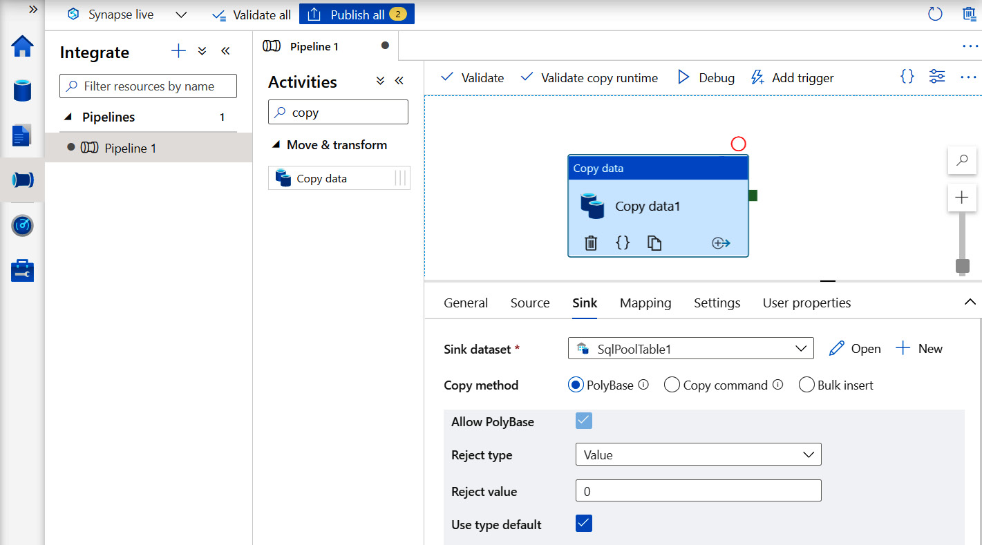
Figure 14.1 – Loading data to a Synapse SQL pool by using the PolyBase copy method within Synapse pipelines

The next section teaches us about index maintenance, which is one of the key ways to keep your indexes healthy and performance optimized for corresponding tables.

Reorganizing and rebuilding indexes

Index maintenance is crucial in keeping your query executions healthy. Sometimes, due to bulk data loading or bad selection of the fill factor, you may end up having index fragmentations, which may lead to bad performance in your query executions. You need to set up a scheduled job to keep track of fragmentation and perform index reorganizing or rebuilding accordingly.

You can use the following SQL code to check for fragmentation:

SELECT S.name as 'Schema',

T.name as 'Table',

I.name as 'Index',

DDIPS.avg_fragmentation_in_percent,

DDIPS.page_count

FROM sys.dm_db_index_physical_stats (DB_ID(), NULL, NULL, NULL, NULL) AS DDIPS

INNER JOIN sys.tables T on T.object_id = DDIPS.object_id

INNER JOIN sys.schemas S on T.schema_id = S.schema_id

INNER JOIN sys.indexes I ON I.object_id = DDIPS.object_id

AND DDIPS.index_id = I.index_id

WHERE DDIPS.database_id = DB_ID()

and I.name is not null

AND DDIPS.avg_fragmentation_in_percent > 0

ORDER BY DDIPS.avg_fragmentation_in_percent desc

If your fragmentation value is more than 30%, consider reorganizing indexes, but if it is beyond 50%, you should rebuild your indexes.

You can use the following SQL script to reorganize/rebuild your indexes:

-- To Rebuild you rindex

ALTER INDEX INDEX_NAME ON SCHEMA_NAME.TABLE_NAME

REBUILD;

-- To Reorganize you rindex

ALTER INDEX INDEX_NAME ON SCHEMA_NAME.TABLE_NAME

REORGANIZE;

Next, we will see how materialized views can help in gaining better performance on a dedicated SQL pool.

Materialized views

You can create standard or materialized views in a Synapse SQL pool. Materialized views provide enhanced performance by storing data on a SQL pool, unlike with standard views. You get pre-computed data stored in a SQL pool in the case of materialized views; however, standard views compute their data each time we use them. But one thing that we should always keep in mind is that materialized views are storing data in your SQL pool, so there will be an extra storage cost involved when using materialized views. We need to decide the trade-off between cost and performance as per our business needs.

The following code will give you a list of all materialized views in your Synapse SQL pool:

SELECT V.name as materialized_view, V.object_id

FROM sys.views V

JOIN sys.indexes I ON V.object_id= I.object_id AND I.index_id < 2;

Next, we can see that the syntax for creating a materialized view is similar to that for a standard view:

CREATE MATERIALIZED VIEW [ schema_name. ] materialized_view_name

    WITH (  

      <distribution_option>

    )

    AS <select_statement>

[;]

<distribution_option> ::=

    {  

        DISTRIBUTION = HASH ( distribution_column_name )  

      | DISTRIBUTION = ROUND_ROBIN  

    }

<select_statement> ::=

    SELECT select_criteria

If you need to improve the performance of a complex query against large data volumes, you can go for materialized views.

Next, we are going to learn how we can enhance query performance by using an appropriate resource class.

Using an appropriate resource class

A resource class is used to determine the performance capacity of a query. By specifying the resource class, you predefine the compute resource limit for query execution in a Synapse SQL pool. There are two types of resource class, and we are going to learn about them in the following sections.

Static resource classes

Static resource classes are ideal for higher concurrency and a constant data volume. These resource classes allocate the same data warehouse units, regardless of the current performance level.

These are the predefined database roles associated with static resource classes:

• staticrc10
• staticrc20
• staticrc30
• staticrc40
• staticrc50
• staticrc60
• staticrc70
• staticrc80

Similar to static resource classes, you can also use dynamic resource classes. Let's learn about these in the next section.

Dynamic resource classes

Dynamic resource classes are ideal for growing or variable amounts of data. These resource classes allocate variable amounts of memory, depending upon the current service level. By default, a smallrc dynamic resource class is assigned to each user.

These are the predefined database roles associated with dynamic resource classes:

• smallrc
• mediumrc
• largerc
• xlargerc

You can run the following script on your SQL pool to add a user to a largec role:

EXEC sp_addrolemember 'largerc', 'newuser'

If you need to remove any user from a largec role in your SQL pool, you can run the following script:

EXEC sp_droprolemember 'largerc', 'newuser';

You can refer to the following link to learn more about resource classes in a Synapse SQL pool: https://docs.microsoft.com/en-us/azure/synapse-analytics/sql-data-warehouse/resource-classes-for-workload-management.

In the next section, we are going to learn about workload management in a SQL pool, which is one of the most important features for managing query performance.

Implementing best practices for a Synapse serverless SQL pool

Some of the best practices discussed in the preceding section will be valid even for a serverless SQL pool; however, there are few other considerations for serverless SQL pools. We are going to learn about some of these recommendations in the following sections.

Selecting the region to create a serverless SQL pool

If you are creating a storage account while creating a Synapse workspace, then your serverless SQL pool and storage account will be created in the same region where you created your workspace. But if you are planning to access other storage accounts, make sure you are creating your workspace in the same region. If you try accessing your data in a different region, there will be some network latency in data movement, but you can avoid this by using the same region for your serverless SQL pool as for your storage account.

You need to keep in mind that once the workspace is created, you cannot change the region of a serverless SQL pool separately.

Files for querying

Although you can query various file types in a serverless SQL pool, you will get better performance if you are using Parquet files. So, if possible, try converting Comma-Separated Values (CSV) files or JavaScript Object Notation (JSON) files in to Parquet files. Parquet is a columnar data storage format that stores binary data in a column-oriented way. These files enable good compression by organizing values of each column adjacently, which makes the file size relatively smaller when compared to CSV or JSON files.

However, if converting CSV to Parquet is not possible for any reason, try to keep the file size between 100 Megabytes (MB) and 10 GB for optimal performance. It is also better to use multiple small files instead of one large file.

Using CETAS to enhance query performance

CETAS is an abbreviated form of CREATE EXTERNAL TABLE .. AS. This operation creates external table metadata and exports the SELECT query result to a set of files in the storage account.

The following code is an example of using CETAS to create an external table:

-- use CETAS to export select statement with OPENROWSET result to  storage

CREATE EXTERNAL TABLE population_by_year_state

WITH (

    LOCATION = 'aggregated_data/',

    DATA_SOURCE = population_ds,  

    FILE_FORMAT = census_file_format

)  

AS

SELECT decennialTime, stateName, SUM(population) AS population

FROM

    OPENROWSET(BULK 'https://azureopendatastorage.blob.core.windows.net/censusdatacontainer/release/us_population_county/year=*/*.parquet',

    FORMAT='PARQUET') AS [r]

GROUP BY decennialTime, stateName

GO

-- you can query the newly created external table

SELECT * FROM population_by_year_state

CETAS generates Parquet files, so statistics are automatically generated when you use the external table for the first time, which helps in improving performance for subsequent queries.

Now that we have learned how to implement best practices for a Synapse SQL pool, in the following section we will learn how to implement best practices for a Synapse Spark pool.

Implementing best practices for a Synapse Spark pool

As with Synapse SQL pools, it is also important to keep our Spark pool healthy. In this section, we are going to learn how to optimize cluster configuration for any particular workload. We will also learn how to use various techniques for enhancing Apache Spark performance.

Configuring the Auto-pause setting

There are some major advantages of using Platform-as-a-Service (PaaS) instead of an on-premises environment, and the Auto-pause setting is one of the best features that PaaS has to offer. If you are running a Spark cluster on your on-premises environment, you need to pay for provisioning it even though you may only need to use this cluster for a couple of hours a day. However, Synapse gives you the option to configure the Auto-pause setting to pause a cluster automatically if not in use. Upon entering a value for the Number of minutes idle field within the Auto-pause setting, the Spark pool will go to a Pause state automatically if it remains idle for the specified duration, as seen in the following screenshot:

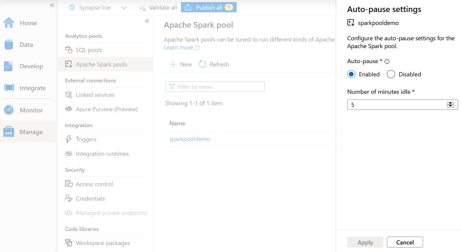
Figure 14.2 – Auto-pause setting for a Synapse Spark pool in the Manage hub of Synapse Studio

When your Spark pool is paused, you are not being charged for the compute power. However, your data is still residing in the storage account even if the Spark pool is paused, hence you are only paying for the data storage.

Next, let's learn some best practices for enhancing Apache Spark performance.

Enhancing Apache Spark performance

In this section of the chapter, we are going to learn how data format, file size, caching, and so on impact job execution performance on the Synapse Spark pool. We will also learn about Spark memory recommendations and how bucketing helps in reducing computational overhead during a job execution on Spark.

So, let's dive into the next section to learn how using an optimal data format can help in getting better Apache Spark performance.

Using an optimal data format

Spark supports various data formats—for example, CSV, JSON, XML, Parquet, Optimized Row Columnar (ORC), and AVRO; however, it is recommended to use Parquet files for better performance. Parquet files are the columnar storage file format of the Apache Hadoop ecosystem. Typically, Spark jobs are Input/Output (I/O)-bound, not Central Processing Unit (CPU)-bound, so a fast compression codec will help in enhancing performance. You can use a Snappy compression with Parquet files for best performance on a Synapse Spark pool.

The following section will outline the use of caching for better performance on Spark.

Using the cache

There are different ways to use caching in Spark, such as persist(), cache(), and CACHE TABLE. Spark uses Cache() and Persist() methods to store the intermediate computation of a Resilient Data Distribution (RDD), DataFrame, and Dataset. This intermediate data can be used for subsequent actions.

The following Scala code is an example of using the cache() method with a DataFrame:

import spark.implicits._

  val columns = Seq("Id","Text")

  val data = Seq(("1", "This is an exmple of Spark DataFrame 

using Cache() method"),

    ("2", "We can replace Cache() with Persist() method in 

this example"))

  val df = data.toDF(columns:_*)

  val dfCache = df.cache()

  dfCache.show(true)

We can replace the cache() method with the persist() method in the preceding example, as illustrated here:

  val dfCache = df.persist()

The following screenshot displays the execution of the code on a Synapse Spark pool:

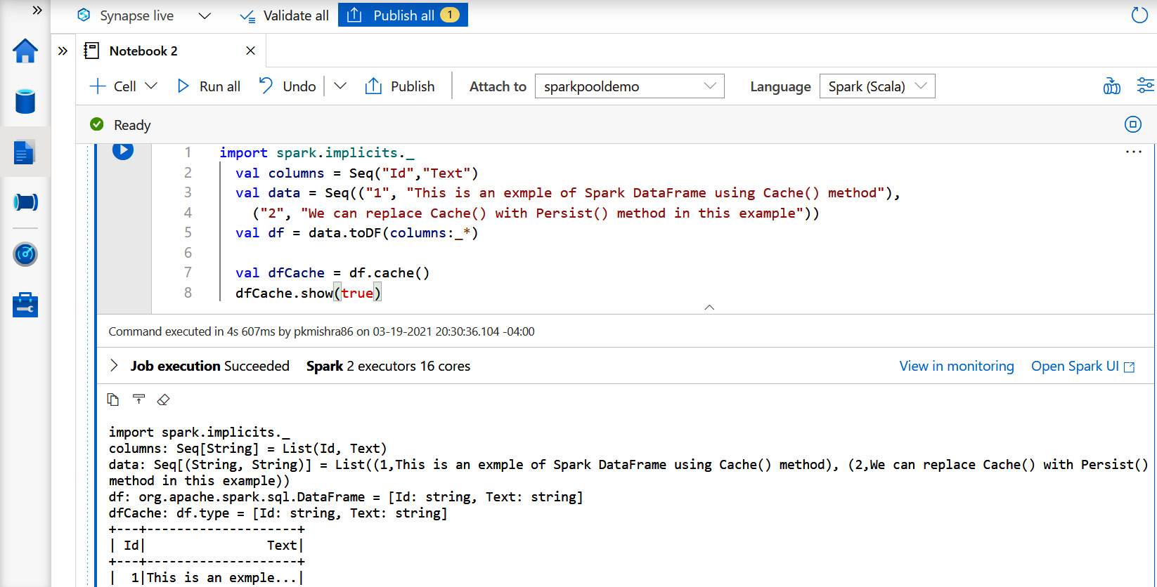
Figure 14.3 – Running Scala code in a notebook within Synapse Studio

We can also use SQL's CACHE TABLE command to create a TableName table in memory. A LAZY keyword can be used with CACHE TABLE to make caching lazy. Lazy cache tables are created only when it is first used, instead of immediately.

The following code will create a CacheTable for the TableName table:

%%sql   

CACHE TABLE CacheTable SELECT * FROM TableName

Similarly, the following code will create a CacheLazyTable table:

%%sql   

CACHE LAZY TABLE CacheLazyTable SELECT * FROM TableName

You can validate the records by running the following script in your Synapse notebook:

%%sql

SELECT * FROM CacheLazyTable

The following screenshot displays the records from CacheLazyTable:

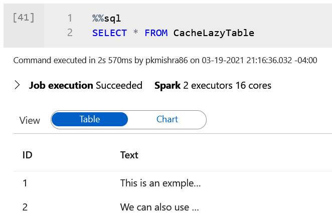
Figure 14.4 – Running a SELECT query against CacheLazyTable using a Synapse Spark pool

Now that we have learned how to create tables in memory for better performance, it's time to learn how to use memory efficiently within a Spark pool.

Spark memory considerations

Spark memory is responsible for storing intermediate state while executing tasks. Apache Spark in Azure Synapse uses Apache Hadoop YARN (where YARN is an acronym for Yet Another Resource Negotiator) to control the memory used by the container in each Spark node. The main job of YARN is to split up the functionalities of the job scheduling into separate daemons. Apache Spark memory is broken into two segments, namely the following:

• Storage memory: Cached data and broadcast variables are stored in storage memory. Spark uses the Least Recently Used (LRU) mechanism to clean up the cache for new cache requests.
• Execution memory: Objects created during the execution of a task are stored here by Spark.

If blocks are not used in execution memory, storage memory can borrow the space from execution memory, and vice versa.

Important note

It is recommended to use DataFrames instead of RDD objects to utilize memory in an optimized way.

The following section outlines how you can enhance the performance of your Spark jobs with the use of bucketing.

Using bucketing

Bucketing is a technique in Spark that is used to optimize the performance of a task. We need to provide the number of buckets for the bucketing column, and the data processing engine will calculate the hash value during the load time to decide which bucket it is going to reside in.

Bucketing can be used to optimize aggregations and joins, which we will learn about in the next section.

Optimizing joins and shuffles

Joins play a critical role when developing a Spark job, so it's important to know about optimizations while working with join operations. Let's try to learn about different join types supported by Apache Spark. These are outlined here:

• SortMerge: Spark uses the SortMerge join type by default, which is a two-step join. First, it sorts the left and right side of the data, and then merges the sorted data from both sides. This join type is best suited for large datasets but may be computationally expensive because of sorting operations. Although this is the default join algorithm in Spark, you can turn it off by setting a False value for the spark.sql.join.preferSortMergeJoin internal parameter.
• Merge: If you are using bucketing, then the Merge join algorithm can be used instead of SortMerge, and you can avoid expensive sort operations on your dataset.
• Shuffle hash join: When the SortMerge join type is turned off, Spark uses the Shuffle hash join type, which works on the concept of map reduce. With a Shuffle hash join, the values of the join column are considered as the output keys, and the DataFrame is shuffled based on these keys. In the end, DataFrames are joined in the reduce phase. It is important to filter out rows that are irrelevant to the keys before joining, in order to avoid unnecessary data shuffling.
• Broadcast: In the case of broadcast joins, the smaller table is broadcasted to all the worker nodes, and because of this it is considered to yield maximum performance in the case of little datasets. We can use the following code to provide a hint to Spark to broadcast a table:

  import org.apache.spark.sql.functions.broadcast

  val dataframe = largedataframe.join(broadcast(smalldataframe), "key")

  Spark maintains the threshold internally to automatically apply broadcast joins based on the table size; however, we can modify the default threshold value of 10 MB to any specific value by using spark.sql.autoBroadcastJoinThreshold.

So far, we have learned about implementing various best practices on a Synapse Spark pool. Now, in the next section, we will learn how to select the correct executor size for Spark jobs.

Selecting the correct executor size

An executor is a process on a worker node that is launched for an application in coordination with the cluster manager. Each application has its own executor, and they are used to run tasks and keep data in memory or disk storage.

The following diagram displays the components of a Spark application:

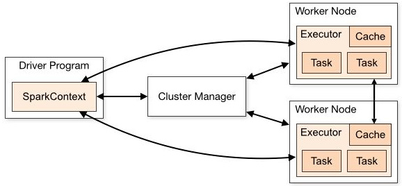
Figure 14.5 – Components of a Spark application

We need to consider the following best practices while working with Spark jobs:

• We should keep the heap size below 32 GB and reduce the number of cores to keep garbage collection overhead below 10%.
• 30 GB per executor is considered the best starting point.
• Increase the number of executor cores for larger clusters.
• For concurrent queries, create multiple parallel Spark applications and distribute queries across these parallel applications.

In this section, we covered the best practices that are common for any Spark jobs, but the list might be even longer based on different specific scenarios.

Summary

This chapter concludes the entire book. In this chapter, we learned about implementing the best practices for Synapse SQL pools and Spark pools. We learned how we keep indexes healthy in a SQL pool such that we gain better performance, and we also learned about using PolyBase and materialized views in Synapse dedicated SQL pools for enhanced performance. This chapter also included the best file type and size to be used in the case of a Synapse serverless SQL pool. Configuring the Auto pause setting to help save costs in terms of computational power was also highlighted in this chapter. Last but not least, we learned about memory considerations and bucketing in a Spark pool.

I am thankful to you for traveling with me on this learning journey. Congratulations on reaching the finish line in this book, and I wish you all the best as you continue exploring Azure Synapse.

Hope to meet you again in my next learning journey!