A.1 Introduction

Descriptions of the models are given starting in Section A.2. First, a few mathematical preliminaries are presented that indicate how the various quantities can be computed.

The incomplete gamma function¹ is given by

with

A useful fact is . Also, define

At times, we will need this integral for nonpositive values of . Integration by parts produces the relationship

This process can be repeated until the first argument of G is , a positive number. Then, it can be evaluated from

However, if is a negative integer or zero, the value of is needed. It is

which is called the exponential integral. A series expansion for this integral is

When is a positive integer, the incomplete gamma function can be evaluated exactly as given in the following theorem.

The incomplete beta function is given by

where

is the beta function, and when (but ), repeated integration by parts produces

where r is the smallest integer such that . The first argument must be positive (that is, ).

Numerical approximations for both the incomplete gamma and the incomplete beta function are available in many statistical computing packages as well as in many spreadsheets, because they are just the distribution functions of the gamma and beta distributions. The following approximations are taken from [2]. The suggestion regarding using different formulas for small and large x when evaluating the incomplete gamma function is from [103]. That reference also contains computer subroutines for evaluating these expressions. In particular, it provides an effective way of evaluating continued fractions.

For , use the series expansion

while for , use the continued-fraction expansion

The incomplete gamma function can also be used to produce cumulative probabilities from the standard normal distribution. Let , where Z has the standard normal distribution. Then, for , , while for , .

The incomplete beta function can be evaluated by the series expansion

The gamma function itself can be found from

For values of above 10, the error is less than . For values below 10, use the relationship

The distributions are presented in the following way. First, the name is given along with the parameters. Many of the distributions have other names, which are noted in parentheses. Next, the density function and distribution function are given. For some distributions, formulas for starting values are given. Within each family, the distributions are presented in decreasing order with regard to the number of parameters. The Greek letters used are selected to be consistent. Any Greek letter that is not used in the distribution means that that distribution is a special case of one with more parameters but with the missing parameters set equal to 1. Unless specifically indicated, all parameters must be positive.

Except for two distributions, inflation can be recognized by simply inflating the scale parameter . That is, if X has a particular distribution, then has the same distribution type, with all parameters unchanged except that is changed to . For the lognormal distribution, changes to with unchanged, while for the inverse Gaussian, both and are multiplied by c.

For several of the distributions, starting values are suggested. They are not necessarily good estimators, but just places from which to start an iterative procedure to maximize the likelihood or other objective function. These are found by either the methods of moments or percentile matching. The quantities used are

For grouped data or data that have been truncated or censored, these quantities may have to be approximated. Because the purpose is to obtain starting values and not a useful estimate, it is often sufficient to just ignore modifications. For three- and four-parameter distributions, starting values can be obtained by using estimates from a special case, then making the new parameters equal to 1. An all-purpose starting value rule (for when all else fails) is to set the scale parameter equal to the mean and set all other parameters equal to 2.

Risk measures may be calculated as follows. For , the Value at Risk, solve the equation . Where there are convenient explicit solutions, they are provided. For , the Tail Value at Risk, use the formula

Explicit formulas are provided in a few cases.

All the distributions listed here (and many more) are discussed in great detail in Kleiber and Kotz [69]. In many cases, alternatives to maximum likelihood estimators are presented.

A.2 The Transformed Beta Family

A.2.1 The Four-Parameter Distribution

A.2.1.1 Transformed Beta –

(generalized beta of the second kind, Pearson Type VI)²

A.2.2 Three-Parameter Distributions

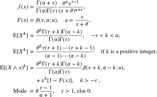
A.2.2.1 Generalized Pareto –

(beta of the second kind)

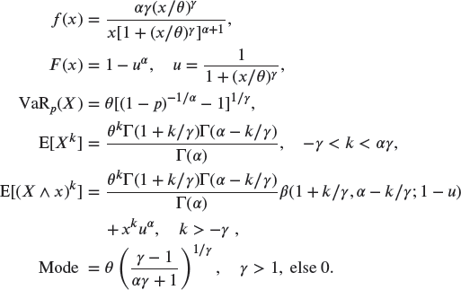
A.2.2.2 Burr –

(Burr Type XII, Singh–Maddala)

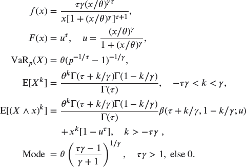
A.2.2.3 Inverse Burr –

(Dagum)

A.2.3 Two-Parameter Distributions

A.2.3.1 Pareto –

(Pareto Type II, Lomax)

A.2.3.2 Inverse Pareto –

A.2.3.3 Loglogistic –

(Fisk)

A.2.3.4 Paralogistic –

This is a Burr distribution with .

Starting values can use estimates from the loglogistic (use for ) or Pareto (use ) distributions.

A.2.3.5 Inverse Paralogistic –

This is an inverse Burr distribution with .

Starting values can use estimates from the loglogistic (use for ) or inverse Pareto (use ) distributions.

A.3 The Transformed Gamma Family

A.3.1 Three-Parameter Distributions

A.3.1.1 Transformed Gamma –

(generalized gamma)

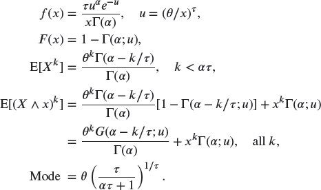
A.3.1.2 Inverse Transformed Gamma –

(inverse generalized gamma)

A.3.2 Two-Parameter Distributions

A.3.2.1 Gamma –

(When and , it is a chi-square distribution with n degrees of freedom.)

A.3.2.2 Inverse Gamma –

(Vinci)

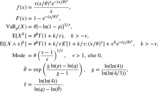
A.3.2.3 Weibull –

A.3.2.4 Inverse Weibull –

(log-Gompertz)

A.3.3 One-Parameter Distributions

A.3.3.1 Exponential –

A.3.3.2 Inverse Exponential –

A.4 Distributions for Large Losses

The general form of most of these distributions has probability starting or ending at an arbitrary location. The versions presented here all use zero for that point. The distribution can always be shifted to start or end elsewhere.

A.4.1 Extreme Value Distributions

A.4.1.1 Gumbel –

( can be negative)

A.4.1.2 Frechet –

This is the inverse Weibull distribution of Section A.3.2.4.

A.4.1.3 Weibull³ –

A.4.2 Generalized Pareto Distributions

A.4.2.1 Generalized Pareto –

This is the Pareto distribution of Section A.2.3.1 with replaced by and replaced by .

A.4.2.2 Exponential –

This is the same as the exponential distribution of Section A.2.3.1 and is the limiting case of the above distribution as .

A.4.2.3 Pareto –

This is the single-parameter Pareto distribution of Section A.5.1.4. From the above distribution, shift the probability to start at .

A.4.2.4 Beta –

This is the beta distribution of Section A.6.1.2 with .

A.5 Other Distributions

A.5.1.1 Lognormal –

( can be negative)

A.5.1.2 Inverse Gaussian –

A.5.1.3 Log-t –

( can be negative) Let Y have a t distribution with r degrees of freedom. Then, has the log-t distribution. Positive moments do not exist for this distribution. Just as the t distribution has a heavier tail than the normal distribution, this distribution has a heavier tail than the lognormal distribution.

A.5.1.4 Single-Parameter Pareto –

Note: Although there appear to be two parameters, only is a true parameter. The value of must be set in advance.

A.6 Distributions with Finite Support

For these two distributions, the scale parameter is assumed to be known.

A.6.1.1 Generalized Beta –

A.6.1.2 Beta –

The case has no special name but is the commonly used version of this distribution.