
Neural nets fall into the Learning category of our taxonomy. In this chapter, we will expand our neural net toolbox with convolution and pooling layers. A general neural net is shown in Figure 10.1. This is a “deep learning” neural net because it has multiple internal layers. Each layer may have a distinct function and form. In the previous chapter, our multi-layer network had multiple layers, but they were all functionally similar and fully connected.

Deep learning neural net.
Convolutional layers (hence the name) – convolves a feature with the input matrix so that the output emphasizes that feature. This finds patterns.
Pooling layers – these reduce the number of inputs to be processed in layers further down the chain.
Fully connected layers
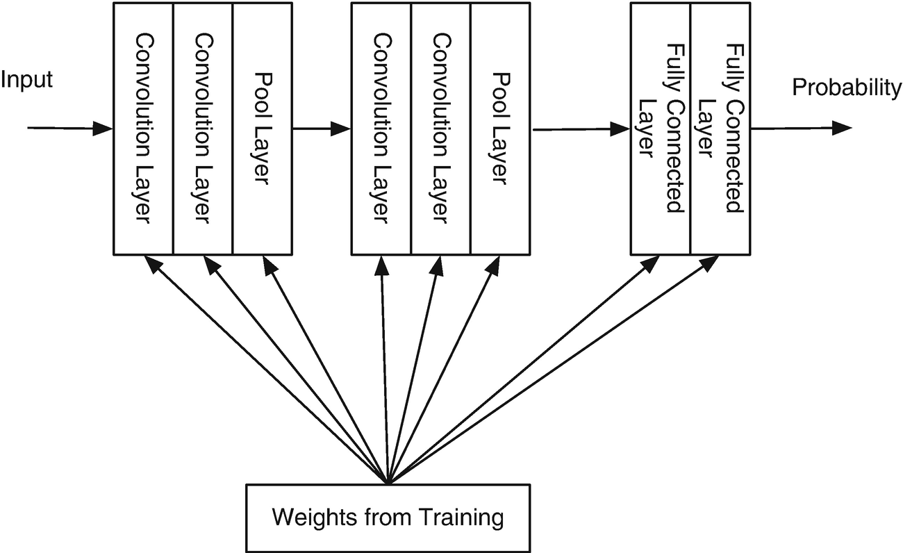
Deep learning convolutional neural net [13].
We can have as many layers as we want. The following recipes will detail each step in the chain. We will start by showing how to gather image data online. We won’t actually use online data, but the process may be useful for your work.
We will then describe the convolution process. The convolution process helps to accent features in an image. For example, if a circle is a key feature, convolving a circle with an input image will emphasize circles.
The next recipe will implement pooling. This is a way of condensing the data. For example, if you have an image of a face, you may not need every pixel. You need to find the major features, mouth and eyes, for example, but may not need details of the person’s iris. This is the reverse of what people do with sketching. A good artist can use a few strokes to clearly represent a face. She then fills in detail in successive passes over the drawing. Pooling, at the risk of losing information, reduces the number of pixels to be processed.
We will then demonstrate the full network using random weights. Finally, we will train the network using a subset of our data and test it on the remaining data, as before.
For this chapter, we are going to use pictures of cats. Our network will produce a probability that a given image is a picture of a cat. We will train networks using cat images and also reuse some of our digit images from the previous chapter.
10.1 Obtain Data Online for Training a Neural Net
10.1.1 Problem
We want to find photographs online for training a cat recognition neural net.
10.1.2 Solution
Use the online database ImageNet to search for images of cats.
10.1.3 How It Works
ImageNet, http://www.image-net.org, is an image database organized according to the WordNet hierarchy. Each meaningful concept in WordNet is called a “synonym set.” There are more than 100,000 sets and 14 million images in ImageNet. For example, type in “Siamese cat.” Click on the link. You will see 445 images. You’ll notice that there are a wide variety of shots from many angles and a wide range of distances.
This is a great resource! However, we are going to instead use pictures of our own cats for our test to avoid copyright issues. The database of photos on ImageNet may prove to be an excellent resource for you to use in training your own neural nets. However, you should review the ImageNet license agreement to determine whether your application can use these images without restrictions.
10.2 Generating Training Images of Cats
10.2.1 Problem
We want grayscale photographs for training a cat recognition neural net.
10.2.2 Solution
Take photographs using a digital camera. Crop them to a standard size manually, then process them using native MATLAB functions to create grayscale images.
10.2.3 How It Works
We first take pictures of several cats. We’ll use them to train the net. The photos are taken using an iPhone 6. We limit the photos to facial shots of the cats. We then frame the shots so that they are reasonably consistent in size and minimize the background. We then convert them to grayscale.
We use the function ImageArray to read in the images. It takes a path to a folder containing the images to be processed. A lot of the code has nothing to do with image processing, just with dealing with unix files in the folder that are not images. ScaleImage is in the file reading loop to scale them. We flip them upside down so that they are the right side up from our viewpoint. We then average the color values to make grayscale. This reduces an n by n by 3 array to n by n. The rest of the code displays the images packed into a frame. Finally, we scale all the pixel values down by 256 so that each value is from 0 to 1. The body of ImageArray is shown in the listing below.
The function has a built-in demo with our local folder of cat images. The images are scaled down by a factor of 24, or 16, so that they are displayed as 64x64 pixel images.
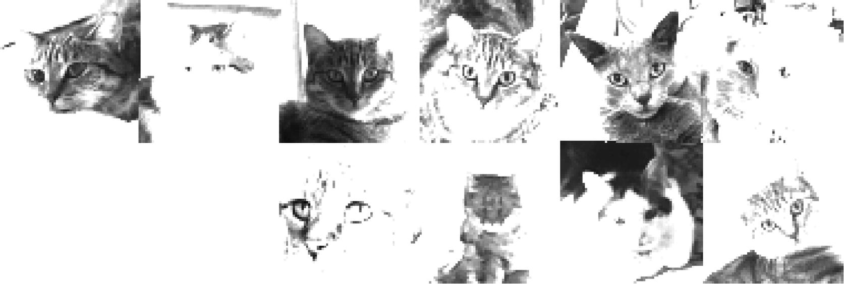
64x64 pixel grayscale cat images.
ImageArray averages the three colors to convert the color images to grayscale. It flips them upside down, since the image coordinates are opposite to that of MATLAB. We used the GraphicConverterTM application to crop the images around the cat face and make them all 1024x1024 pixels. One of the challenges of image matching is to do this process automatically. Also, typically training uses thousands of images. We will be using just a few to see if our neural net can determine if the test image is a cat, or even one we have used in training! ImageArray scales the image using the function ScaleImage, shown below.

Image scaled from 1024x1024 to 256x256.
10.3 Matrix Convolution
10.3.1 Problem
We want to implement convolution as a technique to emphasize key features in images, to make learning more effective. This will then be used in the next recipe to create a convolving layer for the neural net.
10.3.2 Solution
Implement convolution using MATLAB matrix operations.
10.3.3 How It Works

Convolution process showing the mask at the beginning and end of the process.
The mask represents a feature. In effect, we are seeing if the feature appears in different areas of the image. We can have multiple masks. There is one bias and one weight for each element of the mask for each feature. In this case, instead of 16 sets of weights and biases, we only have 4. For large images, the savings can be substantial. In this case, the convolution works on the image itself. Convolutions can also be applied to the output of other convolutional layers or pooling layers, as shown in Figure 10.2.
Convolution is implemented in Convolve.m. The mask is input a and the matrix to be convolved is input b.
The demo, which convolves a 3x3 mask with a 6x6 matrix, produces the following 4x4 matrix output.
10.4 Convolution Layer
10.4.1 Problem
We want to implement a convolution connected layer. This will apply a mask to an input image.
10.4.2 Solution
Use code from Convolve to implement the layer. It slides the mask across the image and the number of outputs is reduced.
10.4.3 How It Works
The “convolution” neural net scans the input with the mask. Each input to the mask passes through an activation function that is identical for a given mask. ConvolutionLayer has its own built-in neuron function shown in the listing.
Figure 10.6 shows the inputs and outputs from the demo (not shown in the listing). The tanh activation function is used in this demo. The weights and biases are random.
The convolution of the mask, which is all ones, is just the sum of all the points that it multiplies. The output is scaled by the number of elements in the mask.
10.5 Pooling to Outputs of a Layer
10.5.1 Problem
We want to pool the outputs of the convolution layer to reduce the number of points we need to process in further layers. This uses the Convolve function created in the previous recipe.
10.5.2 Solution

Inputs and outputs for the convolution layer.
10.5.3 How It Works
Pooling layers take a subset of the outputs of the convolutional layers and pass that on. They do not have any weights. Pooling layers can use the maximum value of the pool or take the median or mean value. Our pooling function has all three as options. The pooling function divides the input into n-by-n subregions and returns an n-by-n matrix.
Pooling is implemented in Pool.m. Notice we use str2func instead of a switch statement. a is the matrix to be pooled, n is the number of pools, and type is the name of the pooling function.
These two demos create four pools from a 4x4 matrix. Each number in the output matrix is a pool of one quarter of the input matrix. It uses the default ’mean’ pool method.
Pool is a neural layer whose activation function is effectively the argument passed to Pool.
10.6 Fully Connected Layer
10.6.1 Problem
We want to implement a fully connected layer.
10.6.2 Solution
Use FullyConnectedNN to implement the network.
10.6.3 How It Works
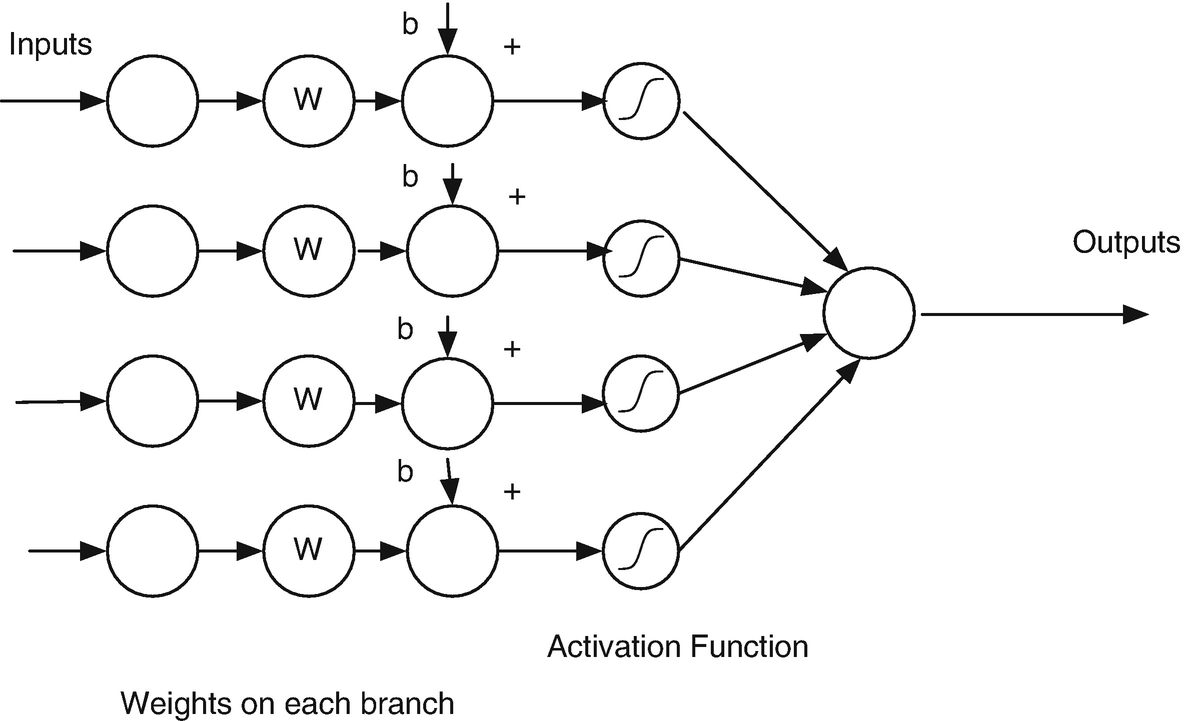
Fully connected neural net. This shows only one output.
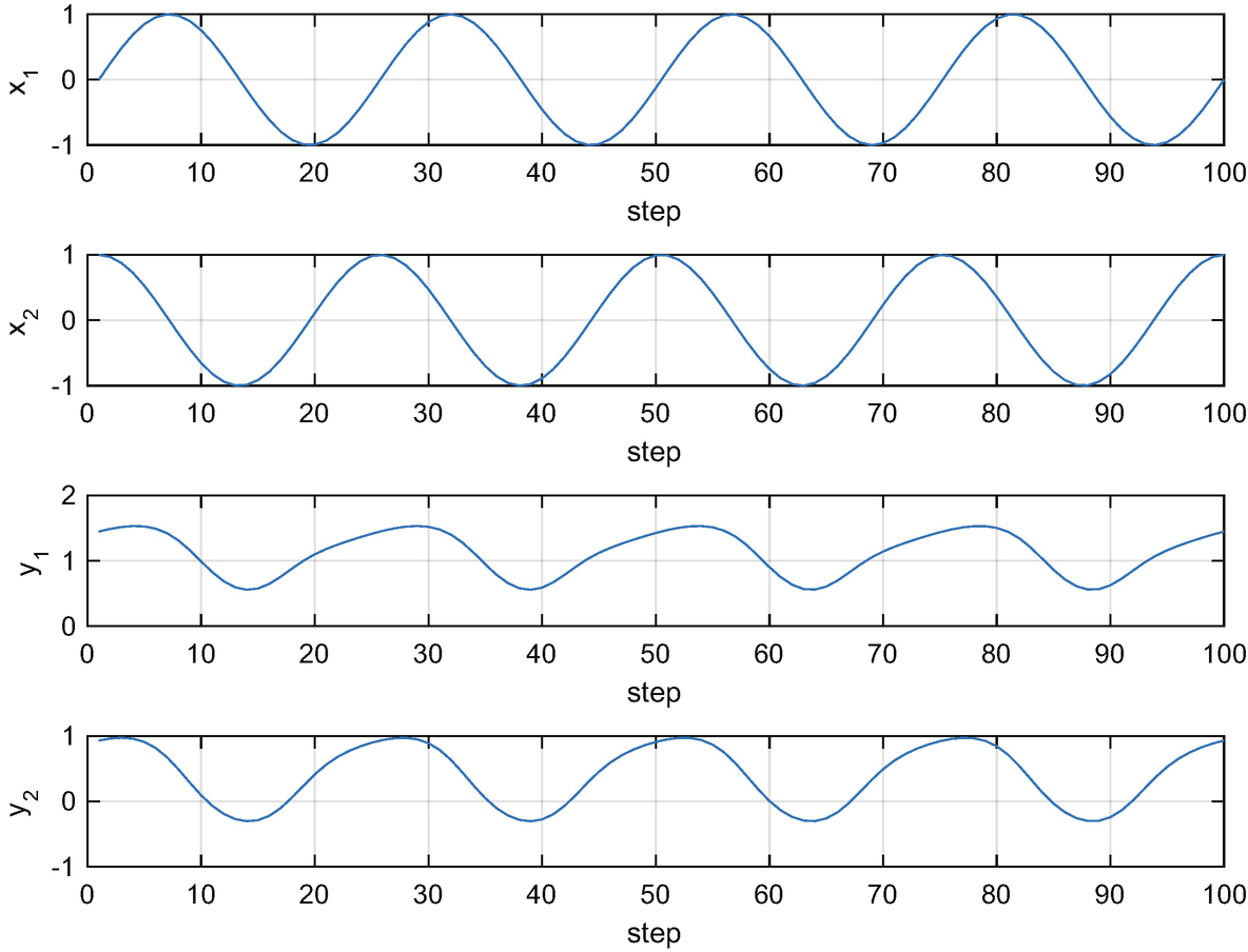
The two outputs from the FullyConnectedNN demo function are shown versus the two inputs.
10.7 Determining the Probability
10.7.1 Problem
We want to calculate a probability that an output is what we expect from neural net outputs.
10.7.2 Solution
Implement the Softmax function. Given a set of inputs, it calculates a set of positive values that add up to 1. This will be used for the output nodes of our network.
10.7.3 How It Works

The function is implemented in Softmax.m.
The built-in demo passes in a short list of outputs.
The results of the demo are:
The last number is the sum of p, which should be (and is) 1.
10.8 Test the Neural Network
10.8.1 Problem
We want to integrate convolution, pooling, a fully connected layer, and Softmax so that our network outputs a probability.
10.8.2 Solution
The solution is to write a convolutional neural net. We integrate the convolution, pooling, fully connected net and Softmax functions. We then test it with randomly generated weights.
10.8.3 How It Works

Neural net for image processing.
ConvolutionNN implements the network. It uses the functions ConvolutionLayer, Pool, FullyConnectedNN and Softmax that we have implemented in the prior recipes. The code in ConvolutionNN, which implements the network, is shown below, in the subfunction NeuralNet. It can generate plots if requested using mesh.
ConvolutionNN has additional subfunctions for defining the data structure and training and testing the network.
We begin by testing the neural net initialized with random weights, using TestNN. This is a script that loads the cat images using ImageArray, initializes a convolutional network with random weights, and then runs it with a selected test image.
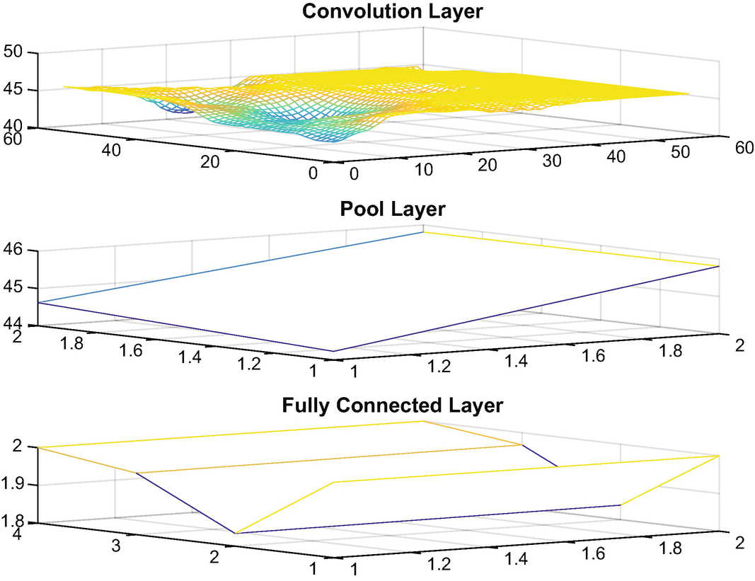
Stages in convolutional neural net processing.
10.9 Recognizing a Number
10.9.1 Problem
We want to determine if an image is that of the number 3.
10.9.2 Solution
We train the neural network with a series of images of the number 3. We then use one picture from the training set and a separate picture and compute the probabilities that they are the number 3.
10.9.3 How It Works
We first run the script Digit3TrainingData to generate a training set. This is a simplified version of the training image generation script in Chapter 5, DigitTrainingData. It only produces one digit, in this case the number 3. input has all 256 bits of an image in a single column. output has the output number 1 for all images. We cycle among three fonts ’times’,’helvetica’,’courier’ for variety. This will make the training more effective when the neural net sees different fonts. Unlike the script in Chapter 4, we store the images as 16x16 pixel images. We also save the three arrays, ’input’, ’trainSets’, ’testSets’ in a .mat file directly using save.
We set rng( ’default’), since fminsearch uses random numbers at times. This makes each run the same. We run the script twice. The first time we use one number for training using the Boolean switch at the top. The second time we use the full training set, like in Chapter 9, setting the Boolean to false. We set tolX = 1e-5. This is the tolerance on the weights, which we are trying to solve. Making it smaller doesn’t improve anything. If you make it really large, like 1, it will degrade the learning. The number of iterations needs to be greater than 10,000. Again, if you make it too small it won’t converge. For one training image, the script returns that the probability of image 2 or 19 being the number 3 is now 80.3% (presumably numbers with the same font). Other test images range from 35.6% to 47.4%.
When we use a lot of images for training representing the various fonts, the probabilities become consistent, though not as high as we would like. Although fminsearch does find reasonable weights we could not say that this network is very accurate.
10.10 Recognizing an Image
10.10.1 Problem
We want to determine if an image is that of a cat.
10.10.2 Solution
We train the neural network with a series of cat images. We then use one picture from the training set and a separate picture reserved for testing and compute the probabilities that they are cats.
10.10.3 How It Works
We run the script TrainNN to see if the input image is a cat. It trains the net from the images in the Cats folder. Many thousands of function evaluations are required for meaningful training, but allowing just a few function evaluations shows that the function is working.
The script returns that the probability of either image being a cat is now 38.8%. This is an improvement considering we only trained it with one image. It took a couple of hours to process.
fminsearch uses a direct search method (Nelder–Mead simplex), and it is very sensitive to initial conditions.
In fact, using this search method poses a fundamental performance barrier for this neural net training, especially for deep learning, where the combinatorics of different weight combos are so big. Better (and faster) results with a global optimization method are likely.
The training code from ConvolutionNN is shown below. It uses MATLAB fminsearch. fminsearch tweaks the gains and biases until it gets a good fit between all the images input and the training image.
Adjust fminsearch parameters.
More images.
More features (masks).
Change the connections in the fully connected layer.
Adding the ability of ConvolutionalNN to handle RGB images directly, rather than converting them to grayscale.
Use a different search method such as a genetic algorithm.
10.11 Summary
Chapter Code Listing
File | Description |
|---|---|
Activation | Generate activation functions. |
ConvolutionalNN | Implement a convolutional neural net. |
ConvolutionLayer | Implement a convolutional layer. |
Convolve | Convolve a 2D array using a mask. |
Digit3TrainingData | Create training data for a single digit. |
FullyConnectedNN | Implement a fully connected neural network. |
ImageArray | Read in images in a folder and convert to grayscale. |
Pool | Pool a 2D array. |
ScaleImage | Scale and image. |
Softmax | Implement the Softmax function. |
TrainNN | Train the convolutional neural net with cat images. |
TrainNNNumber | Train the convolutional neural net on digit images. |
TestNN | Test the convolutional neural net on a cat image. |
TrainingData.mat | Data from TestNN. |