
Chapter 4
Performing Operations by Using Formulas and Functions
MICROSOFT EXAM OBJECTIVES COVERED IN THIS CHAPTER:
- Perform operations by using formulas and functions
- Insert references
- Insert relative, absolute, and mixed references
- Reference named ranges and named tables in formulas
- Calculate and transform datas
- Perform calculations by using the
AVERAGE(),MAX(),MIN(), andSUM()functions - Count cells by using the
COUNT(),COUNTA(), andCOUNTBLANK()functions - Perform conditional operations by using the
IF()function
- Perform calculations by using the
- Format and modify text
- Format text by using
RIGHT(),LEFT(), andMID()functions - Format text by using
UPPER(),LOWER(), andLEN()functions - Format text by using the
CONCAT() andTEXTJOIN()functions
- Format text by using
- Insert references
When you type a formula in a cell, Excel makes it easy to refer to specific cells and ranges. You can add one of three types of references: relative, absolute, and mixed. As you'll see in this chapter, Excel also allows you to refer to a cell range and a table within a workbook.
Next, I will show you how to perform simple calculations and operations using built‐in calculation commands that you type into the Formula Bar. These include calculating the average, minimum, maximum, and sum of a group of cells that contain numbers, counting cells in selected cells or a range, and performing conditional operations with the IF() function.
Finally, you'll learn how to format and modify text in a cell by using a variety of functions. This includes how to return one or more characters at the right, left, or midpoint area with a text string; change text in a cell to uppercase and lowercase; display the number of characters in a text string; and combine text in different strings into one string.
Inserting References
Excel labels each cell with the column letter and then the row number, such as A5. This identification system makes it easy for you to refer to a cell when you enter a formula in another cell. For example, when you're in cell D9 and you want to multiply the number in cell D9 by 3, all you need to type is =(D9*3) in the Formula Bar.
You can create three different types of references:
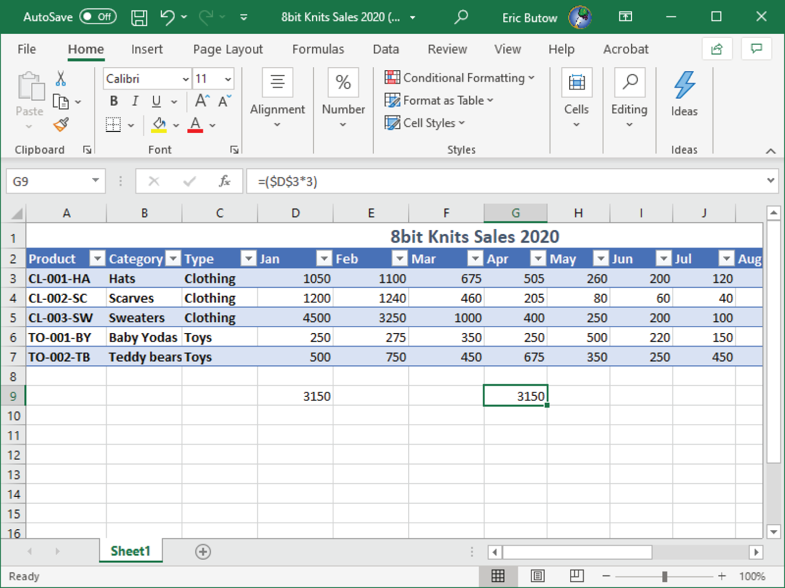
- Relative The default relative cell reference changes when you copy a formula from one cell into another cell. For example, if you type the formula =(D3*3) in cell D9 and then copy cell D9 to cell G9, Excel changes D3 in the formula to G3 because you are now in column G, as shown in the Formula Bar in Figure 4.1.
- Absolute The absolute cell reference contains a dollar sign to the left of the letter and number in the cell that you reference, such as
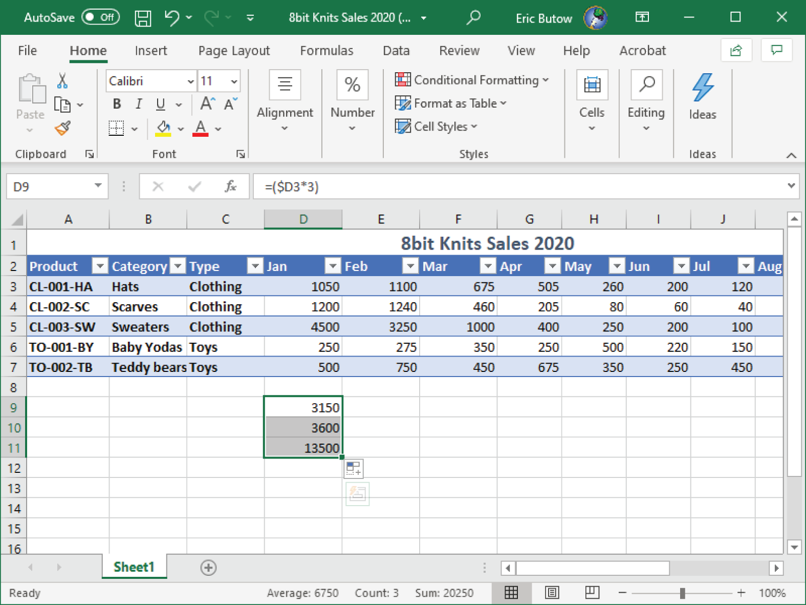
$A$5. When you add an absolute cell reference in a formula, the formula refers to a fixed point in the worksheet. For example, if you type the formula =($D$3*3) in cell D9 and then copy cell D9 to cell G9, cell G9 still calculates the formula using cell D3 (see the Formula Bar in Figure 4.2). - Mixed A mixed cell reference contains a dollar sign to the left of the letter or number in the cell you reference, such as
$A5. When you add a mixed cell reference in a formula, you specify that you want to refer to a value in a fixed column or row in a worksheet. For example, if you type the formula =($D3*3) in cell D9 and then copy cell D9 into cells D10 and D11, Excel multiplies the cells in cells D3, D4, and D5 and places those results in cells D9, D10, and D11, respectively (see Figure 4.3).
FIGURE 4.1 Relative cell reference

Inserting Relative, Absolute, and Mixed References
After you insert a reference into a formula, you may need to change the reference type from one type to another. Excel saves you some time by allowing you to change the reference type quickly. Here's how to do this:
- Create a new workbook and add numbers to cells A1 through A4 in the worksheet.
- In cell A6, type the formula =(A2*5) in the Formula Bar.
FIGURE 4.2 Absolute cell reference
- Press Enter.
- In the Formula Bar, place the cursor to the left or right of A2 in the formula, or between the A and the 2. You know the cell is selected because the cell text A2 turns blue.
- Press F4. The cell turns into the absolute reference
$A$2, as shown in Figure 4.4. - Press F4 again. The cell turns into the mixed reference
A$2. - Press F4 a third time. The cell turns into the mixed reference
$A2. - Press F4 a final time to return the cell to its original relative reference A2.
- Press Esc to exit the Formula Bar.
As you change each formula reference type in the Formula Bar, the new formula also appears in the cell.
FIGURE 4.3 Mixed cell reference
Referencing Named Ranges and Named Tables in Formulas
You don't need to use column names and numbers when you refer to cells in a formula. You can also refer to a named cell range or a named table within a formula. Here is an example that you can follow:
- Open a workbook that has a cell range and a table with numeric values in a worksheet. If you don't have one, refer to previous chapters in this book to create a range and a table.
- Click an empty cell below a column in the table.
- In the Formula Bar, type =SUM( and then start typing the name of the table.
- As you type, a list of potential matches appears in the drop‐down list below the Formula Bar. Double‐click the table name in the list.
FIGURE 4.4 Absolute reference in the Formula Bar

- Now that the table name appears in the formula, start typing the name of the column in the table.
- As you type, a list of potential matches appears in the drop‐down list below the Formula Bar. Double‐click the column name in the list.
- Now that the column name appears in the formula, type ) and then press Enter.
The total of all the numbers within the table appears in the cell, and Excel selects the cell directly below it. When you click the cell in the table, as shown in Figure 4.5, you see the formula in the Formula Bar.
FIGURE 4.5 The formula in the Formula Bar

Calculating and Transforming Datas
Excel includes a variety of built‐in functions for calculating numbers in a spreadsheet to make your life easier. For example, having to average numbers in a column by typing all the numbers within a formula is inefficient at best and tedious at worst.
Let Excel do the work for you when you use one or more of the following calculations in a formula:
- Average
- Maximum value
- Minimum value
- Summation
You may also have times when you need to count instances in a worksheet. For example, you may want to find out how many blank cells are in a worksheet to confirm that you haven't missed adding any important data. Excel includes three counting functions.
If you need to go further and find out how many numeric values reach a certain threshold to meet a condition, such as where numbers are too hot or too cold, Excel includes the IF() function.
Performing Calculations Using the AVERAGE(), MAX(), MIN(), and SUM() Functions
Excel has four standard calculations built in: AVERAGE(), MAX(), MIN(), and SUM(). As with all other calculations you add to a formula, you need to precede any one of these arguments with the equal sign (=) in the Formula Bar.
AVERAGE()
The average is also known as the arithmetic mean, if you remember your middle school math. You can take the average of a group of cells in a worksheet, within a range, or within a table. You can also take an average of two numbers.
Average of Cells
In an empty cell, type =AVERAGE and then the cell range within the worksheet or table in parentheses. For example, if you type =AVERAGE (D3:D7) in the Formula Bar, as shown in the example in Figure 4.6, and then press Enter, the average of all five numbers in the column appears in the cell.
After you press Enter, Excel selects the cell directly below the cell with the average number. Click the cell with the average number to view the formula in the Formula Bar.
Average of Numbers
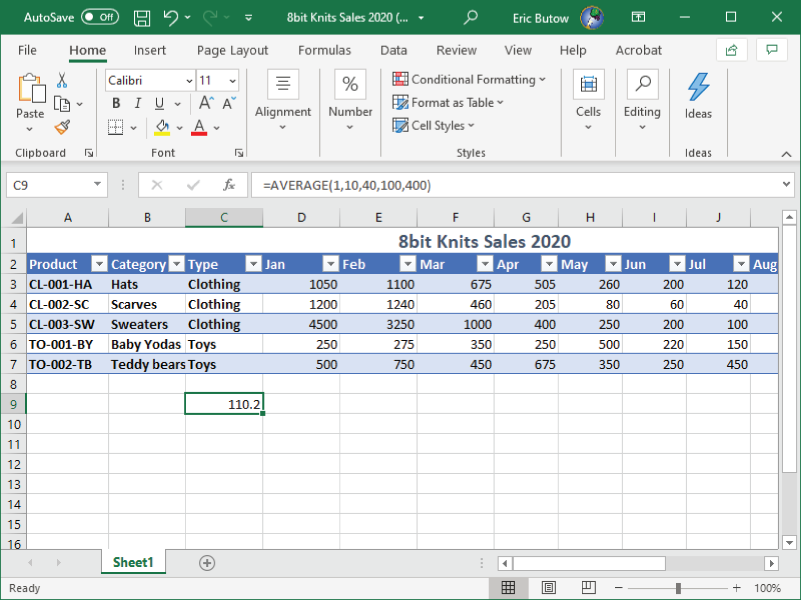
You can average as few as two or as many as 255 numbers by typing =AVERAGE and then entering up to 255 numbers within the parentheses. For example, if you type =AVERAGE(1,10,40,100,400) in the Formula Bar (see Figure 4.7) and then press Enter, the average of all five numbers appears in the cell.
FIGURE 4.6 The average of all five numbers

FIGURE 4.7 Average of five numbers in the cell
MAX()
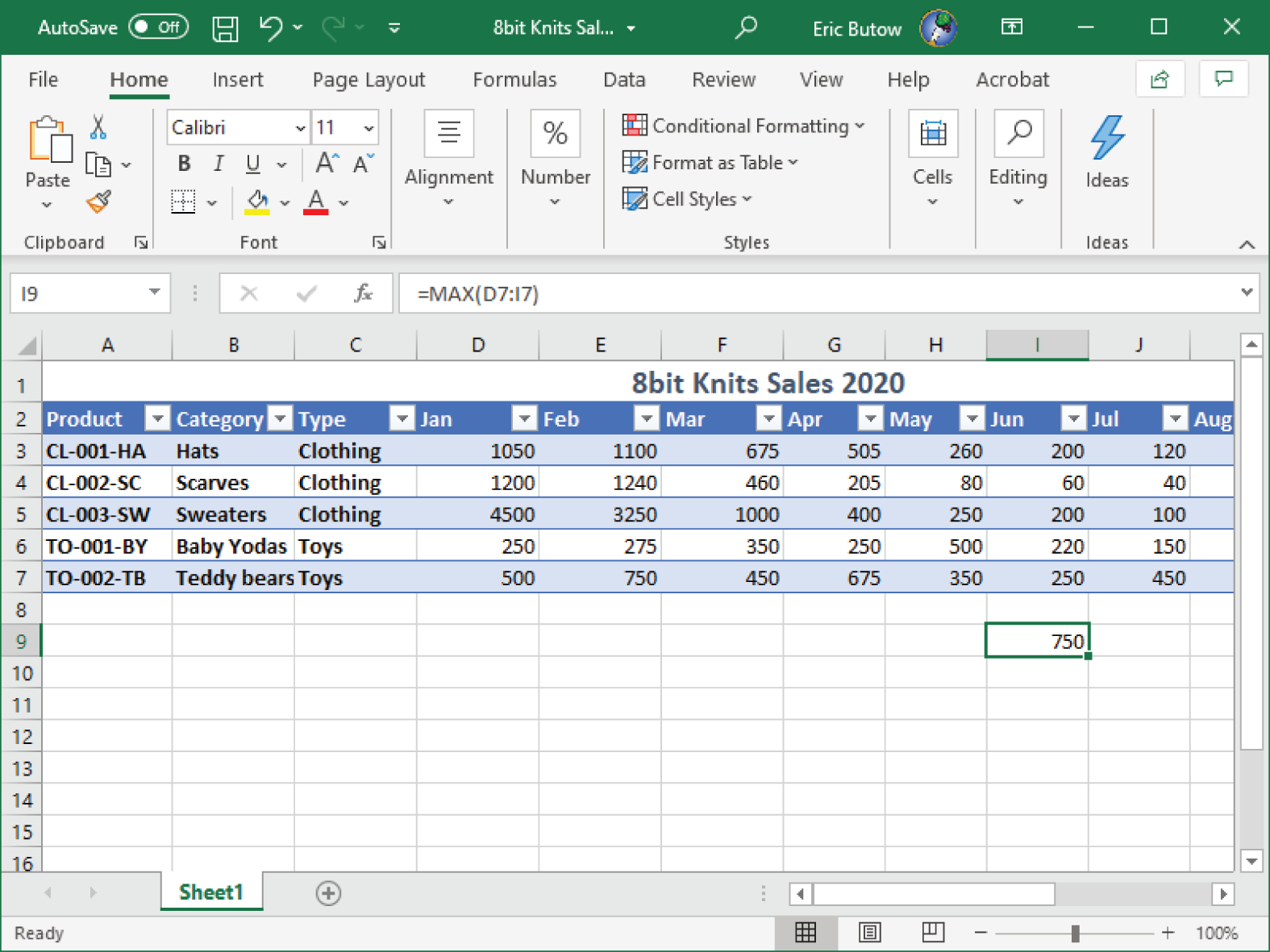
If you need to find the largest number in a range of cells or cells within a table, the MAX() function is the tool you need. After you select a blank cell to add the formula, you can add the MAX() function in the Formula Bar in one of two ways:
- Type =MAX(a,b,c …), where a, b, c, and so on are numbers of your choosing. You can add as many as 255 numbers. When you finish typing the formula, press Enter to see the result in the cell.
- Type =MAX( and then select a range of cells in the worksheet or the table. Excel automatically adds the cell range in your worksheet, so all you have to do is type ) to close the formula and then press Enter. You can see the result in the cell shown in Figure 4.8.
FIGURE 4.8 The calculated MAX result in the cell and the formula in the Formula Bar
MIN()
If you need to find the smallest number in a range of cells or cells within a table, use the MIN() function. After you select a blank cell to add the formula, you can add the MIN() function in the Formula Bar in one of two ways:
- Type =MIN(a,b,c …), where a, b, c, and so on are numbers of your choosing. You can add as many as 255 numbers. When you finish typing the formula, press Enter to see the result in the cell.
- Type =MIN( and then select a range of cells in the worksheet or the table. Excel automatically adds the cell range in your worksheet, so all you have to do is type ) to close the formula and then press Enter. You see the result in the cell (see Figure 4.9).
FIGURE 4.9 The calculated MIN result in the cell and the formula in the Formula Bar

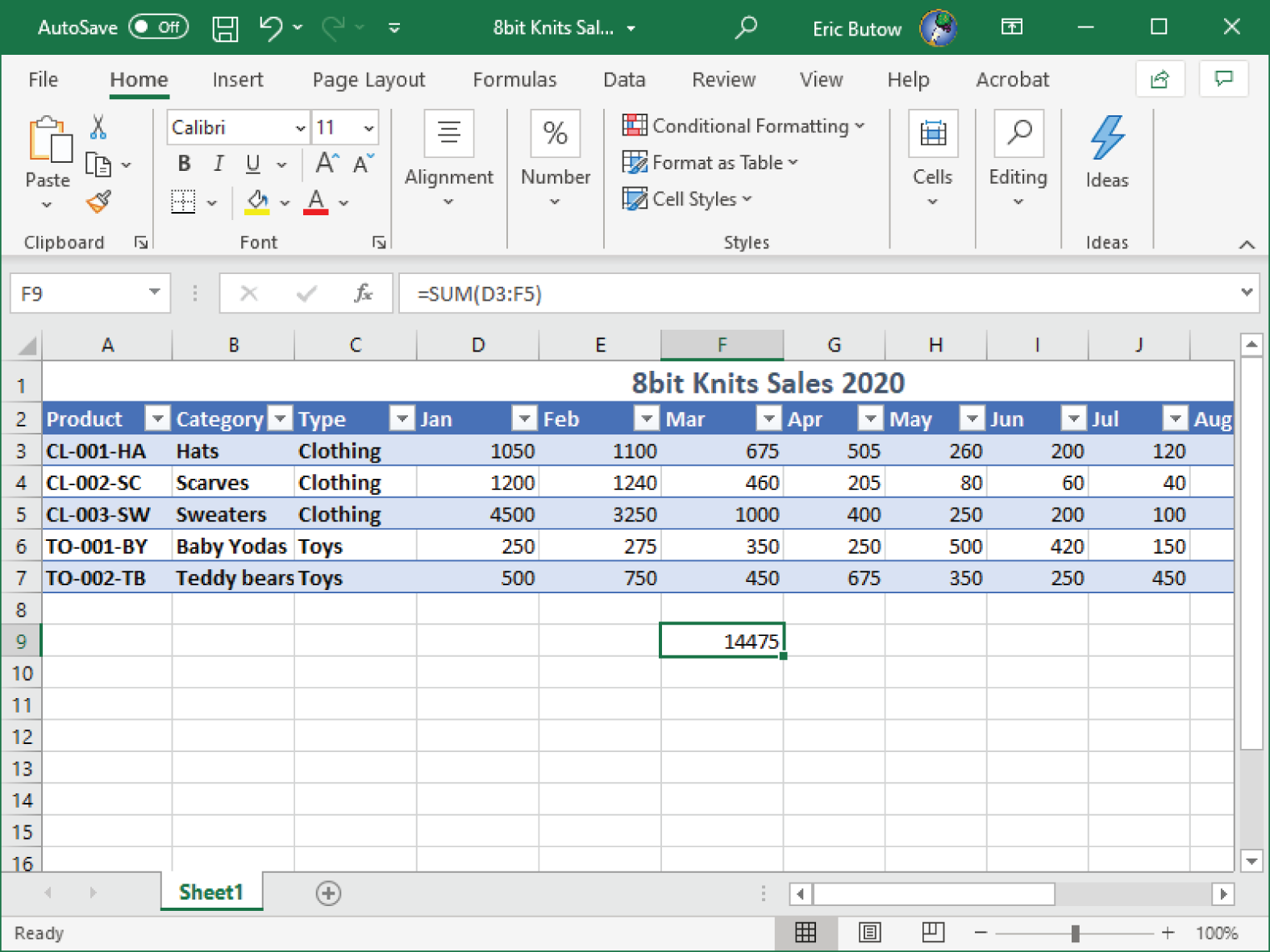
SUM()
When you need to summarize numbers or, more often, numbers in a range of cells, Excel makes this task easy with the SUM() function. After you select a blank cell to add the formula, you can add the SUM() function in the Formula Bar in one of three ways:
- Type =SUM(A1:A5), where you can replace A1:A5 with the starting and ending cells that you want to sum.
- You can sum multiple ranges of cells by typing commas between cell ranges, such as =SUM(A1:A5,D1:D5). When you finish typing the formula, press Enter to see the result in the cell.
- Type =SUM( and then select a range of cells in the worksheet or the table. Excel automatically adds the cell range in your worksheet, so all you have to do is type ) to close the formula and then press Enter. You can see the result in the cell shown in Figure 4.10.
Counting Cells Using the COUNT(), COUNTA(), and COUNTBLANK() Functions
When you need to know how many cells in a worksheet or table have numbers, cells that are not empty, or cells that are empty, you don't have to go through a worksheet or table and count them yourself. You can use the three built‐in counting functions.
FIGURE 4.10 The calculated SUM result in the cell and the formula in the Formula Bar
COUNT()
If you need to count how many cells in a range or cells within a table have numbers, use the COUNT() function. After you select a blank cell to add the formula, you can add the COUNT() function in the Formula Bar in one of three ways:
- Type =COUNT(a,b,c …), where a, b, c, and so on are numbers of your choosing. You can add as many as 255 numbers. When you finish typing the formula, press Enter to see the result in the cell.
- Type =COUNT(A1:A5), where you can replace A1:A5 with the starting and ending cells that you want to count.
- Type =COUNT( and then select a range of cells in the worksheet or the table. Excel automatically adds the cell range in your worksheet, so all you have to do is type ) to close the formula and then press Enter. You can see the result in the cell shown in Figure 4.11.
FIGURE 4.11 The count result in the cell and the formula in the Formula Bar

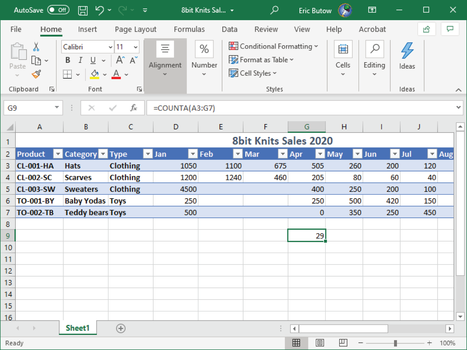
COUNTA()
You can use the COUNTA() function to count the number of cells that are not empty within a range in a worksheet or in a table. After you select a range, add the COUNTA() function in the Formula Bar using one of the following methods:
- Type =COUNTA(a,b,c …), where a, b, c, and so on are numbers of your choosing. You can add as many as 255 numbers. When you finish typing the formula, press Enter to see the result in the cell.
- Type =COUNTA(E1:E5) where you can replace E1:E5 with the starting and ending cells that you want to count.
- Type =COUNT( and then select a range of cells in the worksheet or the table. Excel automatically adds the cell range in your worksheet, so all you have to do is type ) to close the formula and then press Enter. You can see the result in the cell shown in Figure 4.12.
FIGURE 4.12 The COUNTA results in the cell and the formula in the Formula Bar
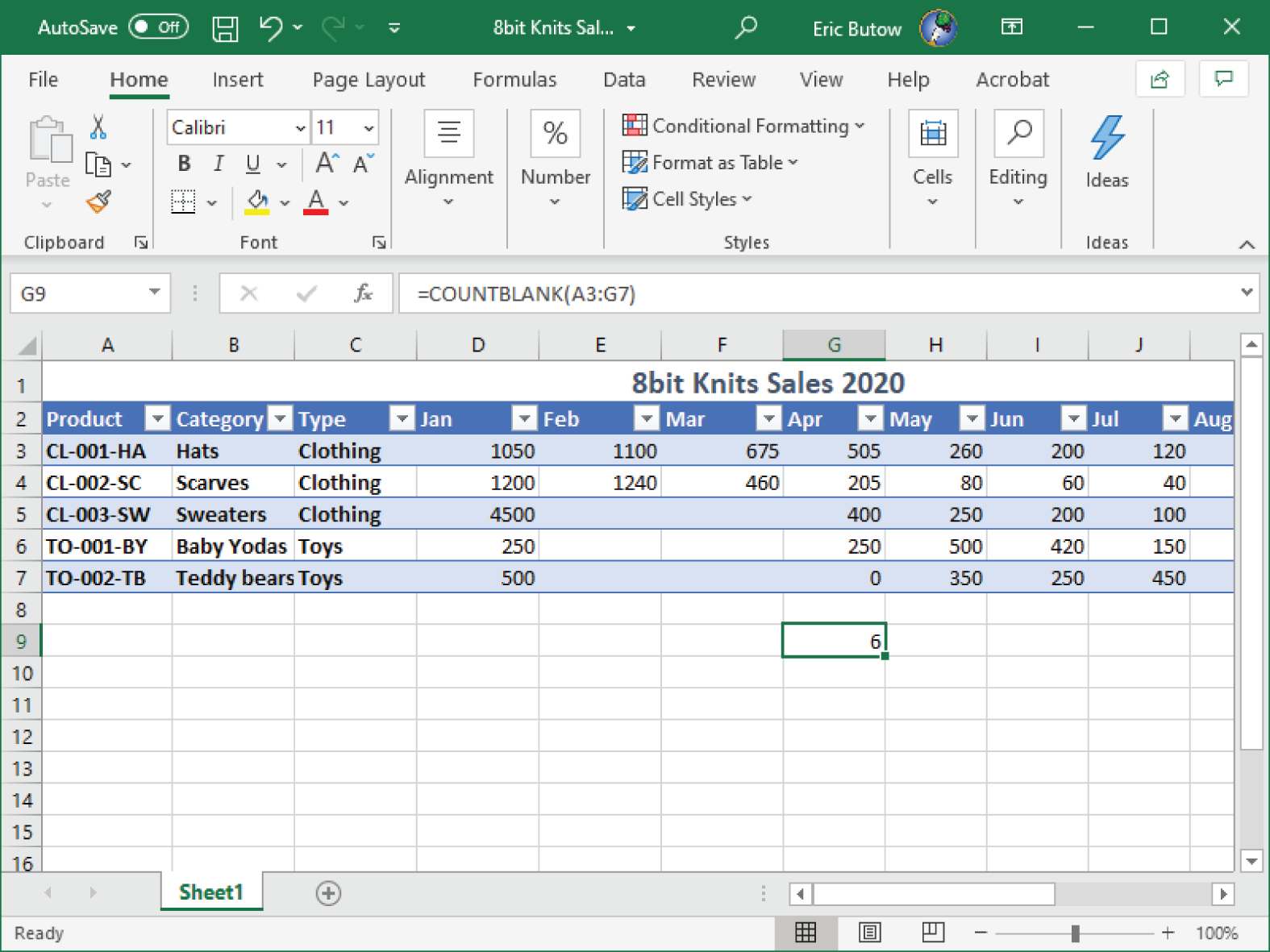
COUNTBLANK()
The COUNTBLANK() function counts the number of empty cells within a selected range in a worksheet or table.
Once you select the range, add the COUNTBLANK() function in the Formula Bar by typing =COUNTBLANK( and then type the cell range, or you can select a range of cells in the worksheet or the table. Excel automatically adds the cell range in your worksheet, so all you have to do is type ) to close the formula and then press Enter. You can see the result in the cell shown in Figure 4.13.
Perform Conditional Operations by Using the IF() Function
If you've ever taken a computer programming class or even used a spreadsheet program before, you know that the if‐then operation is one of the basic operations that you can use to find out if text or a numerical value is true or false.
You can easily add an if‐then condition to a cell in a worksheet or table by using the IF() function. There are two ways to compare values using the IF() function: by having Excel tell you if a cell contains text or a number or if a numeric value meets the condition.
FIGURE 4.13 The calculated COUNTBLANK result in the cell and formula in the Formula Bar
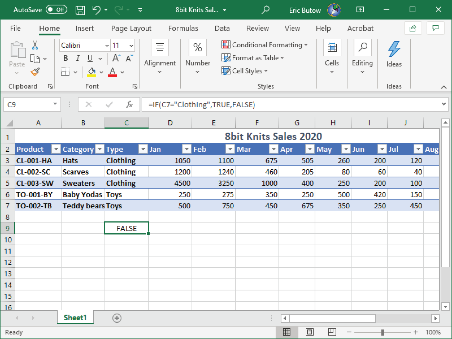
Show if a Cell Contains Text
Here's how to have Excel tell you if a cell contains the text you want to show:
- Place the cursor in cell C9.
- Type =IF(C7="Clothing",true,false) in the Formula Bar.
- Press Enter.
Excel shows FALSE within the cell, as shown in Figure 4.14.
FIGURE 4.14 The FALSE result in the cell with the formula in the Formula Bar
Show if the Numeric Value Meets the Condition
To show that a numeric value meets a certain condition, such as the value in one cell being smaller than another, follow these steps:
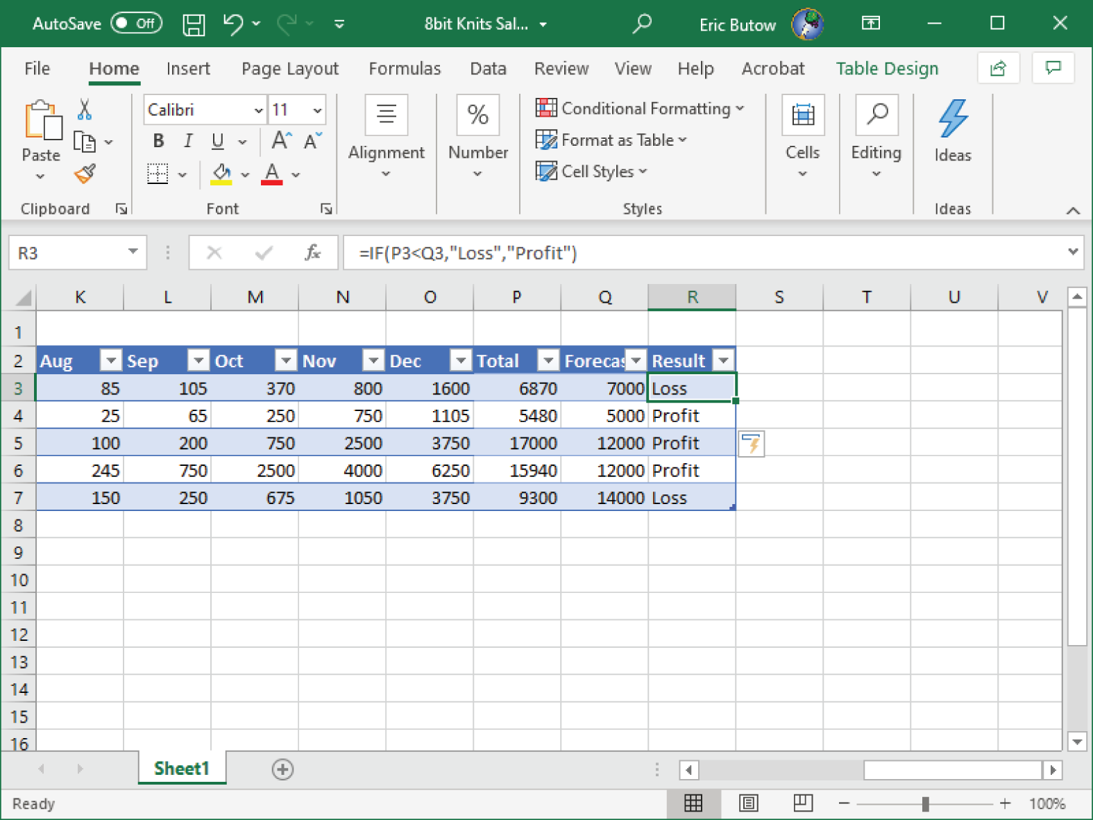
- Click cell R3 in the table.
- Type =IF(P3<Q3,"Loss","Profit") in the Formula Bar. In this formula, Loss is the condition if the comparison is true, and Profit is the condition if the comparison is false.
- Press Enter.
In the table, Excel shows results not only in cell R3 but also within all cells within column R (see Figure 4.15).
Excel copied the formula into all cells, so now you can see if all of the totals in column O when compared with the forecast numbers in column P resulted in a loss or profit for the year.
FIGURE 4.15 The results of the formula in column R
Formatting and Modifying Text
Lists are an effective way of presenting information that readers can digest easily, as demonstrated in this book. Excel includes many powerful tools to create lists easily and then format them so that they look the way you want them to appear.
Formatting Text Using the RIGHT(), LEFT(), and MID() Functions
When you need to extract specific characters from text to place it in another cell, such as only to show a prefix for a part name, you can do so by using the built‐in RIGHT(), LEFT(), and MID() functions that you can add within a formula.
RIGHT()
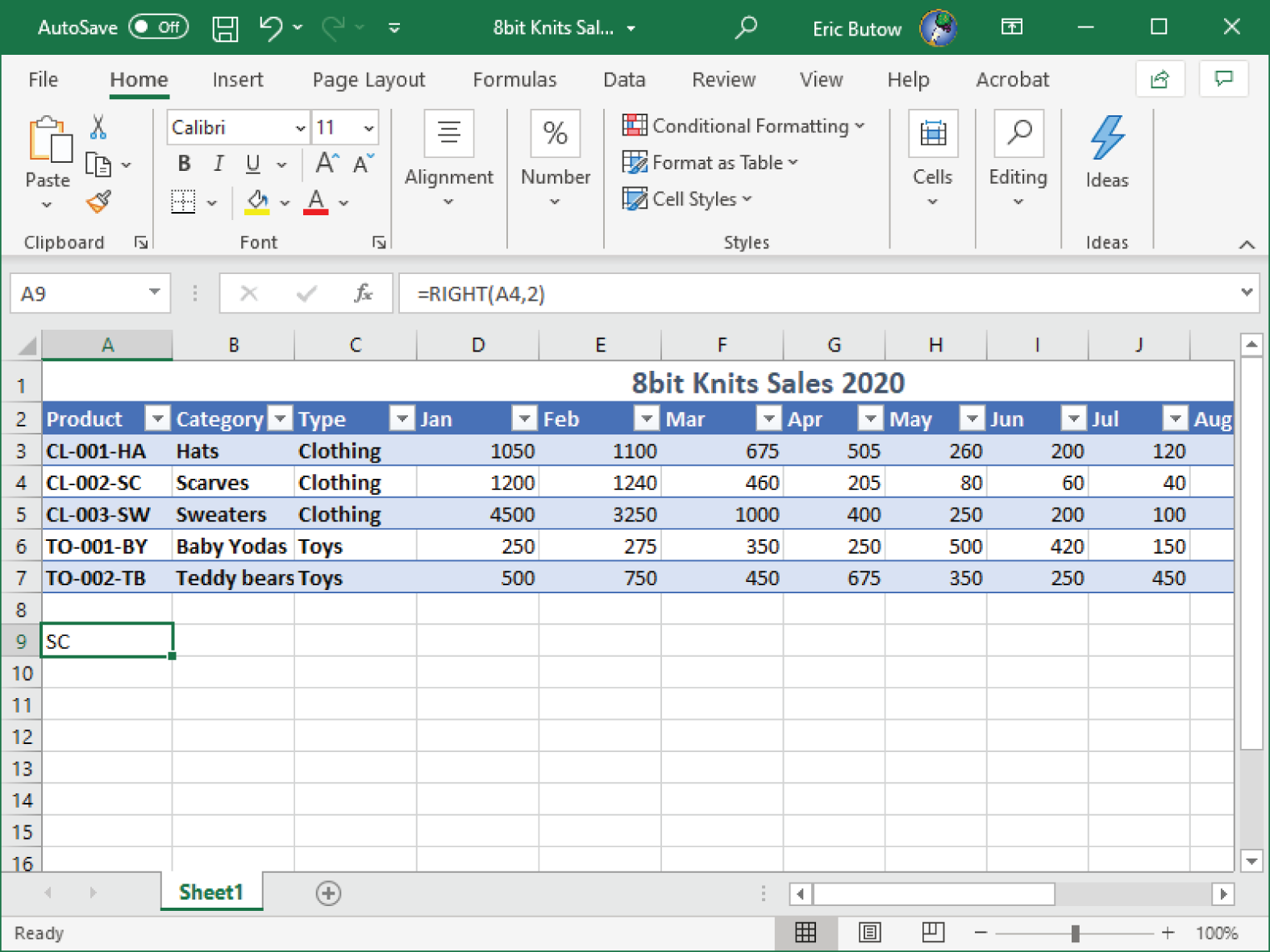
The RIGHT() function shows the last characters in a string of text within a cell in a worksheet or table. Here's how to use the RIGHT() function in a cell:
- Click cell A9 in the table.
- Type =RIGHT(A4,2) in the Formula Bar. A4 is the cell and 2 is the number of characters to show in cell A9.
- Press Enter.
The last two letters in cell A4 appear in cell A9, as shown in Figure 4.16.
FIGURE 4.16 The last two letters in cell A4
LEFT()
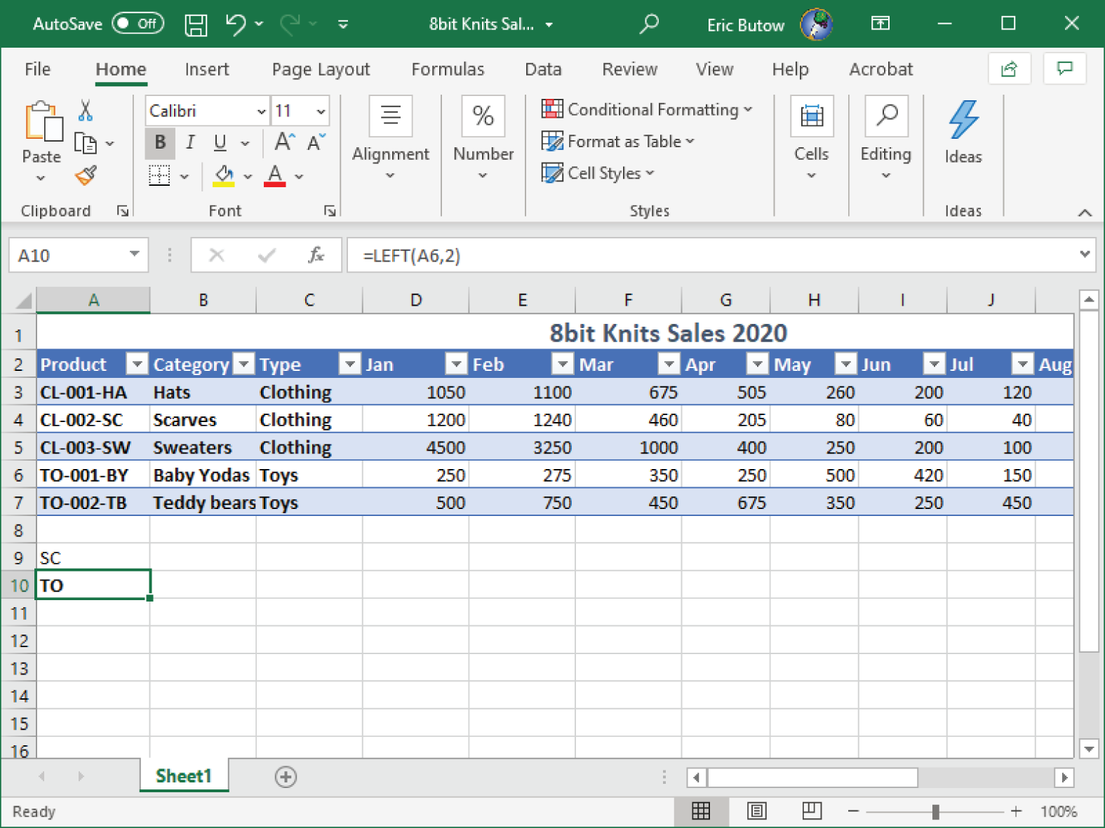
The LEFT() function shows the first characters in a string of text within a cell in a worksheet or table. Use the LEFT() function as demonstrated in the following example:
- Click on cell A10 in the table.
- Type =LEFT(A6,2) in the Formula Bar. A6 is the cell and 2 is the number of characters to show in cell A10.
- Press Enter.
The first two letters in cell A6 appear in cell A10 (see Figure 4.17).
FIGURE 4.17 The first two letters in cell A6
MID()
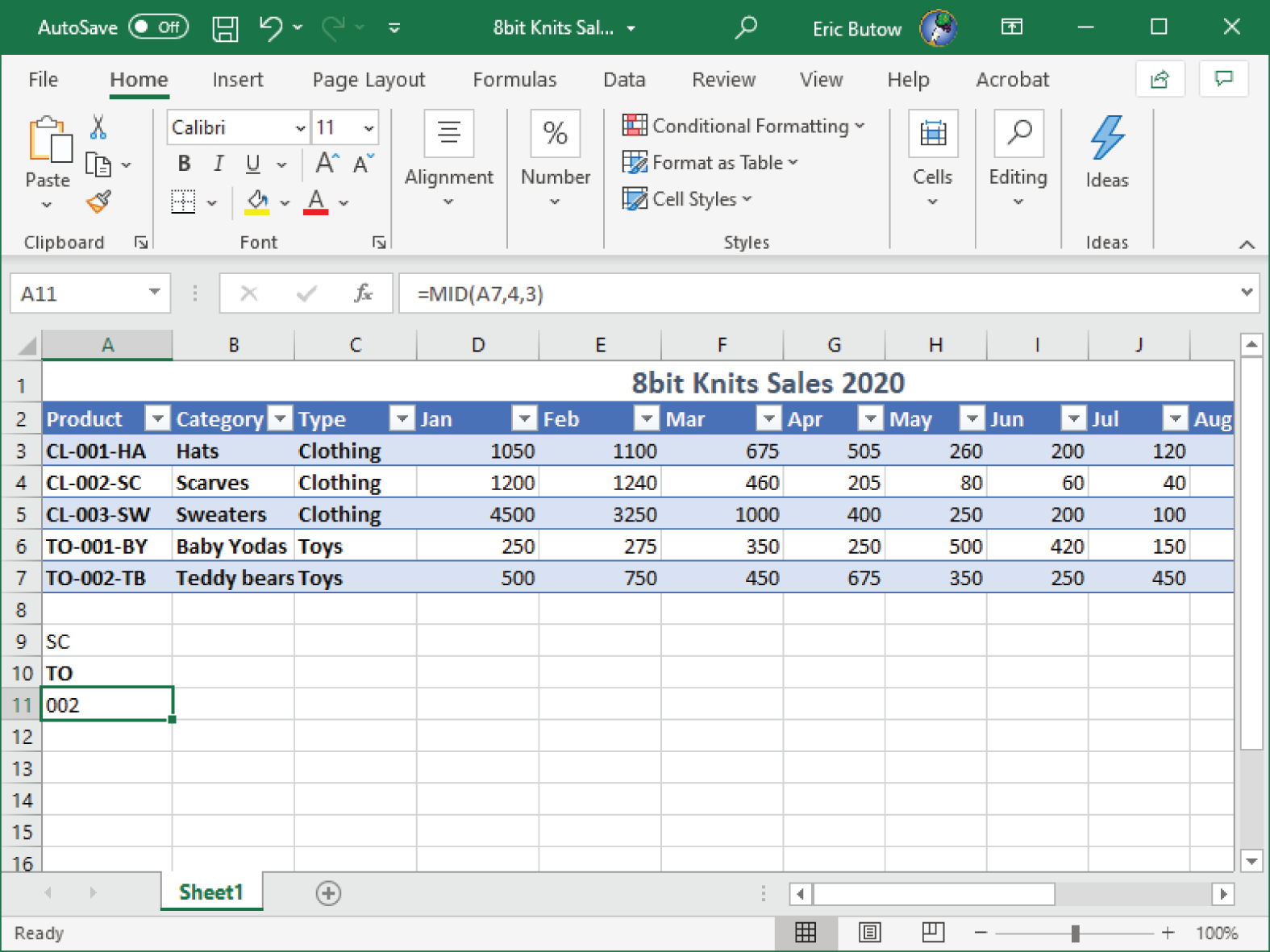
The MID() function shows a specific number of characters in a string of text within a cell in a worksheet or table. Follow these steps to use the MID() function, as shown in the following example:
- Click cell A11 in the table.
- Type =MID(A7,4,3) in the Formula Bar. A6 is the cell, 4 is the fourth character in the text, and 3 is the number of characters to show in cell A11.
- Press Enter.
The three letters starting with the fourth character in cell A7, which is the number 0, appear in cell A11 (see Figure 4.18).
FIGURE 4.18 The three characters in cell A11
Formatting Text Using the UPPER(), LOWER(), and LEN() Functions
When you need to change the text in a cell to all uppercase or all lowercase letters, especially in multiple cells, then that task becomes tedious in no time. Excel has two built‐in features for converting all text in cells within a worksheet or table to uppercase or lowercase.
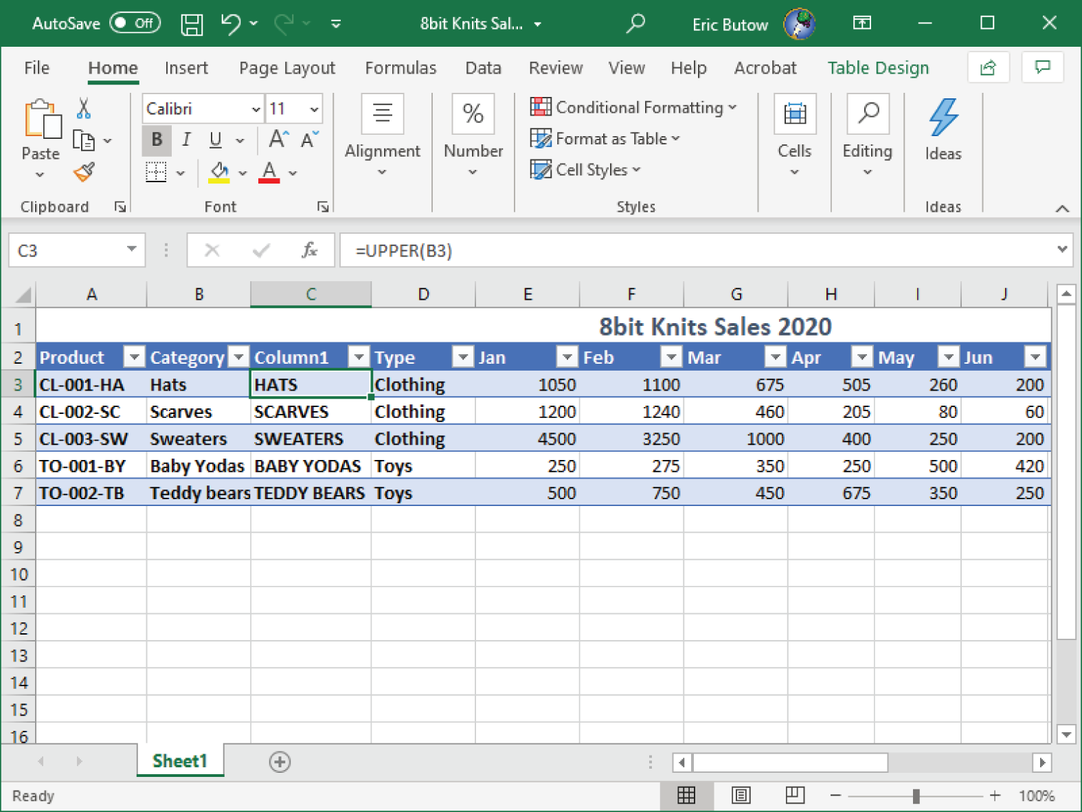
UPPER()
The UPPER() function converts all text in one or more cells to uppercase. Follow these steps to use the UPPER() function:
- Insert a new column to the left of column C.
- Select cell C3.
- Type =UPPER(B3) in the Formula Bar.
- Press Enter.
Excel copies the formula into all cells in column C, so now all text in column B is uppercase in column C (see Figure 4.19).
FIGURE 4.19 All uppercase text in column C
LOWER()
The LOWER() function converts all text in one or more cells to lowercase. Here's how to use the LOWER() function:
- Insert a new column to the left of column C.
- Select cell C3.
- Type =LOWER(B3) in the Formula Bar.
- Press Enter.
Excel copies the formula into all cells in column C, so now all text in column B is lowercase in column C (see Figure 4.20).
FIGURE 4.20 All lowercase text in column C

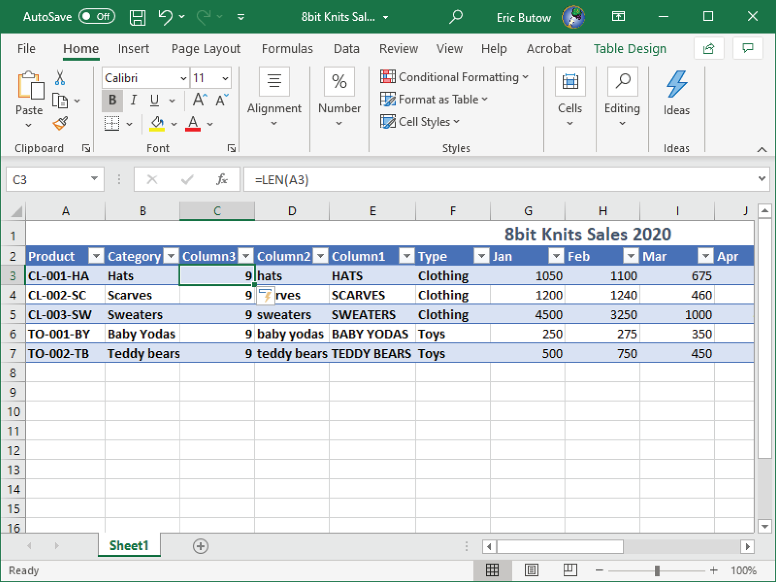
LEN()
The LEN() function, which is short for length, tells you how many characters are in a text string within a cell. For example, you may need to have exactly 14 characters in a product code, and you want to find out which product code has too many or too few characters.
Add the LEN() function in a cell by following these steps:
- Insert a new column to the left of column C.
- Select cell C3.
- Type =LEN(A3) in the Formula Bar.
- Press Enter.
Excel copies the formula into all cells in column C, so the number of characters in cells A3 through A7 appear in column C, and you can confirm that all the product codes have the same length (see Figure 4.21).
FIGURE 4.21 Length in characters in column C
Formatting Text Using the CONCAT() and TEXTJOIN() Functions
When you need to join text from two or more cells and place the joined text into a new cell, Excel gives you two functions to do just that:
CONCAT(), which replaces theCONCATENATE()function in earlier versionsTEXTJOIN(), which is new in Excel 2019 and Excel for Microsoft Office 365
CONCAT()
Adding the CONCAT() function in the Formula Bar doesn't have as many arguments you need to add compared to TEXTJOIN(), but you don't get any options. Follow the steps in this example to see what I mean:
- Click cell B9.
- Type =CONCAT(B3:B4) in the Formula Bar.
- Press Enter.
You see the combined text from cells B3 and B4 in cell B9, as shown in Figure 4.22.
FIGURE 4.22 Combined text with CONCAT() function in the Formula Bar

TEXTJOIN()
When you need to add spaces or another delimiter, such as a comma, between all the words in your combined text, the new TEXTJOIN() function is what you need. Here's how to use TEXTJOIN():
- Click cell B10.
- Type =TEXTJOIN(" ",TRUE,B3:C5) in the Formula Bar. The space between the quotes is a space, and the
TRUEargument tells Excel to ignore any empty cells in the range. - Press Enter.
The combined text in the cell range appears in cell B10 (see Figure 4.23) with a space between each word.
FIGURE 4.23 The combined text with spaces between each text string

Summary
This chapter started by showing you how to insert references in a worksheet or table, including relative, absolute, and mixed references. You also learned how to refer to named ranges and tables within a formula.
After you learned about references, you saw how to perform various calculations using built‐in Excel functions, including the average, maximum, minimum, and sum functions. Then you learned how to count within cells using the three different counting functions in a formula. You also saw how to add the IF() function to perform conditional operations.
Next, I discussed how to format and modify text by using built‐in functions to extract text from the right, left, and middle portions of a text string. You saw how to use functions to change text to all uppercase or all lowercase, as well as get the length of characters in a cell. Finally, you learned how to combine text in two or more cells together using the CONCAT() and TEXTJOIN() functions.
Key Terms
| absolute | mixed | |
| average | references | |
| Formula Bar | relative | |
| maximum | sum | |
| minimum |
Exam Essentials
- Understand how to add relative, absolute, and mixed references in a formula. Know the correct terminology for adding a cell to a formula that will give you relative and absolute results. You must also know how to refer to a named range or table in a worksheet.
- Know how to calculate numbers in one or more cells. Understand how to find the average, maximum, and minimum values in a range of cells that contain numbers. You also need to know how to sum a group of selected cells that have numbers.
- Understand how to count cells. Know how to count the cells in a selected range that have numbers, how many cells are not empty, and how many cells are empty.
- Know how to perform conditional operations. Understand how to determine if a condition is true or false.
- Understand how to extract text from another cell. Know how to use built‐in functions to extract from the right, left, or middle of a string of text in one cell and place the extracted text in another cell.
- Be able to change the case of text and find the length of text in a cell. Know how to change one or more cells to all uppercase letters or all lowercase letters. You also need to understand how to find the length of a text string in one cell and display the length in another cell.
- Know how to join text in two or more cells. Understand how to use the
CONCAT()andTEXTJOIN()functions to join text in two or more cells and know the difference between each function.
Review Questions
- In a formula, how do you change the reference quickly?
- Change the cell reference manually.
- Click the Format icon in the Home ribbon, and then click Format Cells.
- Press F4.
- Right‐click in the Formula Bar, and then click Format Cells.
- What counting function do you use to view all cells in a selected range that have text?
COUNT()COUNTA()COUNTALL()COUNTBLANK()
- What does the function
=RIGHT(A3,5)do?- It shows the first five characters in cell A3.
- It shows the five rows to the right of cell A3.
- It shows the last five characters in cell A3.
- It shows the first three characters and last five characters of all cells with text in column A.
- What are the three reference types? (Choose all that apply.)
- Mixed
- Name
- Relative
- Absolute
- What happens when you try to calculate the average of a range of cells when one or more cells does not have a number in it?
- The function treats the empty cell as the number 0.
- The result of the function is an error message.
- The function returns the number 0.
- The function ignores the empty cells.
- What happens when you show the first five characters of a text string that includes a space?
- Excel ignores the space.
- Excel shows a dialog box with an error message.
- An error message appears in the cell.
- Excel shows the space.
- A2 is what type of cell reference in a formula?
- Absolute
- Relative
- None
- Mixed
- What do you type first in a formula?
- The formula name
- The left parenthesis
- The equal sign
- A colon
- What function do you use when you want to combine text in two cells and not have a space between the combined text?
CONCAT()TEXTJOIN()SUM()COUNT()
- What do you do when you want to summarize cells in multiple ranges?
- Type each
SUM()formula for each range separated by a comma. - Add all of the cells individually within the parentheses in the
SUM()formula. - Type each
SUM()formula for each range separated by a plus (+) sign. - Add a comma between each cell range within the parentheses in the formula.
- Type each