
Chapter 15
Working with Linear Models the Easy Way
IN THIS CHAPTER
Illustrating linear models for regression and classification
Preparing the right data for linear models
Limiting the influence of less useful and redundant variables
Selecting effective feature subsets
Learning from big data by stochastic gradient descent
You can’t complete an overview of basic machine learning algorithms without discovering the linear models family, a common and excellent type of starting algorithm to use when trying to make predictions from data. Linear models comprise a wide family of models derived from statistical science, although just two of them, linear regression and logistic regression, are frequently mentioned and used.
Statisticians, econometricians, and scientists from many disciplines have long used linear models to confirm their theories by means of data validation and to obtain practical predictions. You can find an impressive number of books and papers about this family of models stocked in libraries and universities. This mass of literature discusses many applications as well as the sophisticated tests and statistical measures devised to check and validate the applicability of linear models to many types of data problems in detail.
Machine learning adherents adopted linear models early. However, because learning from data is such a practical discipline, machine learning separates linear models from everything related to statistics and keeps only the mathematical formulations. Statistics powers the models using stochastic descent — the optimization procedure discussed in Chapter 10. The result is a solution that works effectively with most learning problems (although preparing the data requires some effort). Linear models are easy to understand, fast to create, a piece of cake to implement from scratch, and, by using some easy tricks, they work even with big data problems. If you can master linear and logistic regression, you really have the equivalent of a Swiss Army knife for machine learning that can’t do everything perfectly but can serve you promptly and with excellent results in many occurrences.
Starting to Combine Variables
Regression boasts a long history in different domains: statistics, economics, psychology, social sciences, and political sciences. Apart from being capable of a large range of predictions involving numeric values, binary and multiple classes, probabilities, and count data, linear regression also helps you to understand group differences, model consumer preferences, and quantify the importance of a feature in a model.
Stripped of most of its statistical properties, regression remains a simple, understandable, yet effective algorithm for the prediction of values and classes. Fast to train, easy to explain to nontechnical people, and simple to implement in any programming language, linear and logistic regression are the first choice of most machine learning practitioners when building models to compare with more sophisticated solutions. People also use them to figure out the key features in a problem, to experiment, and to obtain insight into feature creation.
Linear regression works by combining through numeric feature summation. Adding a constant number, called the bias, completes the summation. The bias represents the prediction baseline when all the features have values of zero. Bias can play an important role in producing default predictions, especially when some of your features are missing (and so have a zero value). Here’s the common formula for a linear regression:
In this expression, y is the vector of the response values. Possible response vectors are the prices of houses in a city or the sales of a product, which is simply any answer that is numeric, such as a measure or a quantity. The X symbol states the matrix of features to use to guess the y vector. X is a matrix that contains only numeric values. The Greek letter alpha (α) represents the bias, which is a constant, whereas the letter beta (β) is a vector of coefficients that a linear regression model uses with the bias to create the prediction.
 Using Greek letters alpha and beta in regression is widespread to the point that most practitioners call the vector of coefficients the regression beta.
You can make sense of this expression in different ways. To make things simpler, you can imagine that X is actually composed of a single feature (described as a predictor in statistical practice), so you can represent it as a vector named x. When only one predictor is available, the calculation is a simple linear regression. Now that you have a simpler formulation, your high school algebra and geometry tell you that the formulation y=bx+a is a line in a coordinate plane made of an x axis (the abscissa) and a y axis (the ordinate).
When you have more than one feature (a multiple linear regression), you can’t use a simple coordinate plane made of x and y anymore. The space now spans multiple dimensions, with each dimension being a feature. Now your formula is more intricate, composed of multiple x values, each weighted by its own beta. For instance, if you have four features (so that the space is four-dimensional), the regression formulation, as explicated from matrix form, is
This complex formula, which exists in a multidimensional space, isn’t a line anymore, but rather a plane with as many dimensions as the space. This is a hyperplane, and its surface individuates the response values for every possible combination of values in the feature dimensions.
This discussion explains regression in its geometrical meaning, but you can also view it as just a large weighted summation. You can decompose the response into many parts, each one referring to a feature and contributing to a certain portion. The geometric meaning is particularly useful for discussing regression properties, but the weighted summation meaning helps you understand practical examples better. For instance, if you want to predict a model for advertising expenditures, you can use a regression model and create a model like this:
In this formulation, sales are the sum of advertising expenditures, number of shops distributing the product, and the product’s price. You can quickly demystify linear regression by explaining its components. First, you have the bias, the constant a, which acts as a starting point. Then you have three feature values, each one expressed in a different scale (advertising is a lot of money, price is some affordable value, and shops is a positive number), each one rescaled by its respective beta coefficient.
Each beta presents a numeric value that describes the intensity of the relationship to the response. It also has a sign that shows the effect of a change in feature. When a beta coefficient is near zero, the effect of the feature on the response is weak, but if its value is far from zero, either positive or negative, the effect is significant and the feature is important to the regression model.
 To obtain an estimate of the target value, you scale each beta to the measure of the feature. A high beta provides more or less effect on the response depending on the scale of the feature. A good habit is to standardize the features (by subtracting the mean and dividing by standard deviation) to avoid being fooled by high beta values on small-scale features and to compare different beta coefficients. The resulting beta values are comparable, allowing you to determine which ones have the most impact on the response (those with the largest absolute value).
If beta is positive, increasing the feature will increase the response, whereas decreasing the feature will decrease the response. Conversely, if beta is negative, the response will act contrary to the feature: When one is increasing, the other is decreasing. Each beta in a regression represents an impact. Using the gradient descent algorithm discussed in Chapter 10, linear regression can find the best set of beta coefficients (and bias) to minimize a cost function given by the squared difference between the predictions and the real values:
This formula tells you the cost J as a function of w, the vector of coefficients of the linear model. The cost is the summed squared difference of response values from predicted values (the multiplication Xw) divided by two times the number of observations (n). The algorithm strives to find the minimum possible solution values for the difference between the real target values and the predictions derived from the linear regression.
You can express the result of the optimization graphically as the vertical distances between the data points and the regression line. The regression line represents the response variable well when the distances are small, as shown in Figure 15-1. If you sum the squares of the distances, the sum is always the minimum possible when you calculate the regression line correctly. (No other combination of beta will result in a lower error.)
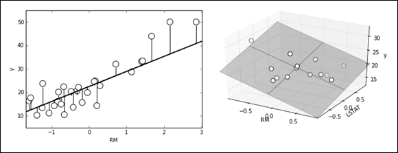
FIGURE 15-1: An example of visualizing errors of a regression line and plane.
In statistics, practitioners often refer to linear regression as ordinary least squares (OLS), indicating a particular way of estimating the solution based on matrix calculus. Using this approach isn’t always feasible. It depends on the computation of the data matrix inversion, which isn’t always possible. In addition, matrix inverse computations are quite slow when the input matrix is large. In machine learning, you obtain the same results using the radient descent optimization, which handles larger amounts of data easier and faster, thus estimating a solution from any input matrix.
R versions of linear and logistic regression heavily rely on the statistical approach. Python versions, such as those found in the Scikit-learn package, use gradient descent. For this reason, the book illustrates examples of linear models using Python.
The only requirement for gradient descent is to standardize (zero mean and unit variance) or normalize (feature values bound between +1 and –1) the features because the optimization process is sensitive to differently scaled features. Standard implementations implicitly standardize (so you don’t have to remember this detail). However, if you use sophisticated implementations, scaling can turn into a serious issue. As a result, you should always standardize the predictors. Gradient descent calculates the solution by optimizing the coefficients slowly and systematically. It bases its update formula on the mathematical derivative of the cost function:
The single weight wj, relative to the feature j, is updated by subtracting from it a term consisting of a difference divided by the number of examples (n) and a learning factor alpha, which determines the impact of the difference in the resulting new wj. (A small alpha reduces the update effect.) The part of the formula that reads (Xw –y) calculates the difference between the prediction from the model and the value to predict. By calculating this difference, you tell the algorithm the size of the prediction error. The difference is then multiplied by the value of the feature j. The multiplication of the error by the feature value enforces a correction on the coefficient of the feature proportional to the value of the feature itself. Because the features pool into a summation, the formula won’t work with efficacy regardless of whether you’re mixing features of different scale — the larger scale will dominate the summation. For instance, mixing measures expressed in kilometers and centimeters isn’t a good idea in gradient descent, unless you transform them using standardization.
Math is part of machine learning, and sometimes you can’t avoid learning formulas because they prove useful for understanding how algorithms work. After demystifying complex matrix formulas into sets of summations, you can determine how algorithms work under the hood and act to ensure that the algorithm engine works better by having the right data and correctly set parameters.
The following Python example uses the Boston dataset from Scikit-learn to try to guess the Boston housing prices using a linear regression. The example also tries to determine which variables influence the result more. Beyond computational issues, standardizing the predictors proves quite useful if you want to determine the influential variables.
from sklearn.datasets import load_bostonfrom sklearn.preprocessing import scaleboston = load_boston()X, y = scale(boston.data), boston.target
The regression class in Scikit-learn is part of the linear_model module. Because you previously scaled the X variables, you don’t need to decide any other preparations or special parameters when using this algorithm.
from sklearn.linear_model import LinearRegressionregression = LinearRegression()regression.fit(X,y)
Now that the algorithm is fitted, you can use the score method to report the R2 measure.
print (regression.score(X,y))0.740607742865
R2, also known as coefficient of determination, is a measure ranging from 0 to 1. It shows how using a regression model is better in predicting the response than using a simple mean. The coefficient of determination is derived from statistical practice and directly relates to the sum of squared errors. You can calculate the R2 value by hand using the following formula:
The upper part of the division represents the usual difference between response and prediction, whereas the lower part represents the difference between the mean of the response and the response itself. You square and sum both differences across the examples. In terms of code, you can easily translate the formulation into programming commands and then compare the result with what the Scikit-learn model reports:
import numpy as npmean_y = np.mean(y)squared_errors_mean = np.sum((y-mean_y)**2)squared_errors_model = np.sum((y – regression.predict(X))**2)R2 = 1- (squared_errors_model / squared_errors_mean)print (R2)0.740607742865
In this case, the R2 on the previously fitted data is around 0.74, which, from an absolute point of view, is quite good for a linear regression model (values over 0.90 are very rare and are sometimes even indicators of problems such as data snooping or leakage).
Because R2 relates to the sum of squared errors and represents how data points can represent a line in a linear regression, it also relates to the statistical correlation measure. Correlation in statistics is a measure ranging from +1 to –1 that tells how two variables relate linearly (that is, if you plot them together, they tell how the lines resemble each other). When you square a correlation, you get a proportion of how much variance two variables share. In the same way, no matter how many predictors you have, you can also compute R2 as the quantity of information explained by the model (the same as the squared correlation), so getting near 1 means being able to explain most of the data using the model.
Calculating the R2 on the same set of data used for the training is common in statistics. In data science and machine learning, you’re always better off to test scores on data that is not used for training. Complex algorithms can memorize the data rather than learn from it. In certain circumstances, this problem can also happen when you’re using simpler models, such as linear regression.
To understand what drives the estimates in the multiple regression model, you have to look at the coefficients_ attribute, which is an array containing the regression beta coefficients. By printing the boston.DESCR attribute, you can understand the variable reference.
print ([a+':'+str(round(b,1)) for a, b in zip(boston.feature_names, regression.coef_,)])['CRIM:-0.9', 'ZN:1.1', 'INDUS:0.1', 'CHAS:0.7', 'NOX:-2.1', 'RM:2.7', 'AGE:0.0', 'DIS:-3.1', 'RAD:2.7', 'TAX:-2.1', 'PTRATIO:-2.1', 'B:0.9', 'LSTAT:-3.7']
The DIS variable, which contains the weighted distances to five employment centers, has the largest absolute unit change. In real estate, a house that’s too far away from people’s interests (such as work) lowers the value. Instead, AGE or INDUS, which are both proportions that describe the building’s age and whether nonretail activities are available in the area, don’t influence the result as much; the absolute value of their beta coefficients is much lower.
Mixing Variables of Different Types
Quite a few problems arise with the effective, yet simple, linear regression tool. Sometimes, depending on the data you use, the problems are greater than the benefits of using this tool. The best way to determine whether linear regression will work is to use the algorithm and test its efficacy on your data.
Linear regression can model responses only as quantitative data. When you need to model categories as a response, you must turn to logistic regression, covered later in the chapter. When working with predictors, you do best by using continuous numeric variables; although you can fit both ordinal numbers and, with some transformations, qualitative categories.
A qualitative variable might express a color feature, such as the color of a product, or a feature that indicates the profession of a person. You have a number of options for transforming a qualitative variable by using a technique such as binary encoding (the most common approach). When making a qualitative variable binary, you create as many features as classes in the feature. Each feature contains zero values unless its class appears in the data, when it takes the value of one. This procedure is called one-hot encoding (as previously mentioned in Chapter 9). A simple Python example using the Scikit-learn preprocessing module shows how to perform one-hot encoding:
from sklearn.preprocessing import OneHotEncoder, LabelEncoderlbl = LabelEncoder()enc = OneHotEncoder()qualitative = ['red', 'red', 'green', 'blue', 'red', 'blue', 'blue', 'green']labels = lbl.fit_transform(qualitative).reshape(8,1)print(enc.fit_transform(labels).toarray())[[ 0. 0. 1.] [ 0. 0. 1.] [ 0. 1. 0.]
[ 1. 0. 0.] [ 0. 0. 1.] [ 1. 0. 0.] [ 1. 0. 0.] [ 0. 1. 0.]]
In statistics, when you want to make a binary variable out of a categorical one, you transform all the levels but one because you use the inverse matrix computation formula, which has quite a few limitations. In machine learning you use gradient descent, so you instead transform all the levels.
If a data matrix is missing data and you don’t deal with it properly, the model will stop working. Consequently, you need to impute the missing values (for instance, by replacing a missing value with the mean value calculated from the feature itself). Another solution is to use a zero value for the missing case, and to create an additional binary variable whose unit values point out missing values in the feature. In addition, outliers (values outside the normal range) disrupt linear regression because the model tries to minimize the square value of the errors (also called residuals). Outliers have large residuals, thus forcing the algorithm to focus more on them than on regular points.
The greatest linear regression limitation is that the model is a summation of independent terms, because each feature stands alone in the summation, multiplied only by its own beta. This mathematical form is perfect for expressing a situation in which the features are unrelated. For instance, a person’s age and eye color are unrelated terms because they do not influence each other. Thus, you can consider them independent terms and, in a regression summation, it makes sense that they stay separated. On the other hand, a person’s age and hair color aren’t unrelated, because aging causes hair to whiten. When you put these features in a regression summation, it’s like summing the same information. Because of this limitation, you can’t determine how to represent the effect of variable combinations on the outcome. In other words, you can’t represent complex situations with your data. Because the model is made of simple combinations of weighted features, it expresses more bias than variance in its predictions. In fact, after fitting the observed outcome values, the solution proposed by linear models is always a proportionally rescaled mix of features. Unfortunately, you can’t represent some relations between a response and a feature faithfully by using this approach. On many occasions, the response depends on features in a nonlinear way: Some feature values act as hurdles, after which the response suddenly increases or decreases, strengthens or weakens, or even reverses.
As an example, consider how human beings grow in height from childhood. If observed in a specific age range, the relationship between age and height is somehow linear: The older the child gets, the taller he or she is. However, some children grow more (overall height) and some grow faster (growth in a certain amount of time). This observation holds when you expect a linear model to find an average answer. However, after a certain age, children stop growing and the height remains constant for a long part of life, slowly decreasing in later age. Clearly, a linear regression can’t grasp such a nonlinear relationship. (In the end, you can represent it as a kind of parabola.)
Another age-related example is the amount spent for consumer products. People in the earliest phases of their life tend to spend less. Expenditures increase during the middle of life (maybe because of availability of more income or larger expenses because of family obligations), but they decrease again in the latter part life (clearly another nonlinear relationship). Observing and thinking more intensely of the world around us shows that many nonlinear relationships exist.
Because the relation between the target and each predictor variable is based on a single coefficient, you don’t have a way to represent complex relations like a parabola (a unique value of x maximizing or minimizing the response), an exponential growth, or a more complex nonlinear curve unless you enrich the feature. The easiest way to model complex relations is by employing mathematical transformations of the predictors using polynomial expansion. Polynomial expansion, given a certain degree d, creates powers of each feature up to the d-power and d-combinations of all the terms. For instance, if you start with a simple linear model such as the following Python code:
and then use a polynomial expansion of the second degree, that model becomes
You make the addition to the original formulation (the expansion) using powers and combinations of the existing predictors. As the degree of the polynomial expansion grows, so does the number of derived terms. The following Python example uses the Boston dataset (found in previous examples) to check the technique’s effectiveness. If successful, the polynomial expansion will catch nonlinear relationships in data and overcome any nonseparability (the problem seen with the perceptron algorithm in Chapter 12) at the expense of an increased number of predictors.
from sklearn.preprocessing import PolynomialFeaturesfrom sklearn.cross_validation import train_test_splitpf = PolynomialFeatures(degree=2)poly_X = pf.fit_transform(X)X_train, X_test, y_train, y_test = train_test_split(poly_X, y, test_size=0.33, random_state=42)from sklearn.linear_model import Ridgereg_regression = Ridge(alpha=0.1, normalize=True)reg_regression.fit(X_train,y_train)print ('R2: %0.3f' % r2_score(y_test,reg_regression.predict(X_test)))R2: 0.819
Because feature scales are enlarged by power expansion, standardizing the data after a polynomial expansion is a good practice.
Polynomial expansion doesn’t always provide the advantages demonstrated by the previous example. By expanding the number of features, you reduce the bias of the predictions at the expense of increasing their variance. Expanding too much may hinder the capability of the model to represent general rules, making it unable to perform predictions using new data. This chapter provides evidence of this issue and a working solution in the section “Solving overfitting by using selection,” which discusses variable selection.
Switching to Probabilities
Up to now, the chapter has considered only regression models, which express numeric values as outputs from data learning. Most problems, however, also require classification. The following sections discuss how you can address both numeric and classification output.
Specifying a binary response
A solution to a problem involving a binary response (the model has to choose from between two possible classes) would be to code a response vector as a sequence of ones and zeros (or positive and negative values, just as the perceptron does). The following Python code proves both the feasibility and limits of using a binary response.
a = np.array([0, 0, 0, 0, 1, 1, 1, 1])b = np.array([1, 2, 3, 4, 5, 6, 7, 8]).reshape(8,1)from sklearn.linear_model import LinearRegressionregression = LinearRegression()regression.fit(b,a)print (regression.predict(b)>0.5)[False False False False True True True True]
In statistics, linear regression can’t solve classification problems because doing so would create a series of violated statistical assumptions. So, for statistics, using regression models for classification purposes is mainly a theoretical problem, not a practical one. In machine learning, the problem with linear regression is that it serves as a linear function that’s trying to minimize prediction errors; therefore, depending on the slope of the computed line, it may not be able to solve the data problem.
When a linear regression is given the task of predicting two values, such as 0 and +1, which are representing two classes, it will try to compute a line that provides results close to the target values. In some cases, even though the results are precise, the output is too far from the target values, which forces the regression line to adjust in order to minimize the summed errors. The change results in fewer summed deviance errors but more misclassified cases.
Contrary to the perceptron example in Chapter 12, linear regression doesn’t produce acceptable results when the priority is classification accuracy, as shown in Figure 15-2. Therefore, it won’t work satisfactorily in many classification tasks. Linear regression works best on a continuum of numeric estimates. However, for classification tasks, you need a more suitable measure, such as the probability of class ownership.
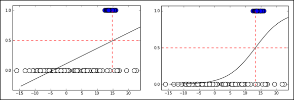
FIGURE 15-2: Probabilities do not work as well with a straight line as they do with a sigmoid curve.
Thanks to the following formula, you can transform linear regression numeric estimates into probabilities that are more apt to describe how a class fits an observation:
In this formula, the target is the probability that the response y will correspond to the class 1. The letter r is the regression result, the sum of the variables weighted by their coefficients. The exponential function, exp(r), corresponds to Euler’s number e elevated to the power of r. A linear regression using this transformation formula (also called a link function) for changing its results into probabilities is a logistic regression.
Logistic regression is the same as a linear regression except that the y data contains integer numbers indicating the class relative to the observation. So, using the Boston dataset from the Scikit-learn datasets module, you can try to guess what makes houses in an area overly expensive (median values >= 40):
from sklearn.linear_model import LogisticRegressionfrom sklearn.cross_validation import train_test_splitbinary_y = np.array(y >= 40).astype(int)X_train, X_test, y_train, y_test = train_test_split(X, binary_y, test_size=0.33, random_state=5)logistic = LogisticRegression()logistic.fit(X_train,y_train)from sklearn.metrics import accuracy_scoreprint('In-sample accuracy: %0.3f' % accuracy_score(y_train, logistic.predict(X_train)))print('Out-of-sample accuracy: %0.3f' % accuracy_score(y_test, logistic.predict(X_test)))In-sample accuracy: 0.973Out-of-sample accuracy: 0.958
The example splits the data into training and testing sets, enabling you to check the efficacy of the logistic regression model on data that the model hasn’t used for learning. The resulting coefficients tell you the probability of a particular class’s being in the target class (which is any class encoded using a value of 1). If a coefficient increases the likelihood, it will have a positive coefficient; otherwise, the coefficient is negative.
for var,coef in zip(boston.feature_names, logistic.coef_[0]): print ("%7s : %7.3f" %(var, coef))
Reading the results on your screen, you can see that in Boston, criminality (CRIM) has some effect on prices. However, the level of poverty (LSTAT), distance from work (DIS), and pollution (NOX) all have much greater effects. Moreover, contrary to linear regression, logistic regression doesn’t simply output the resulting class (in this case a 1 or a 0) but also estimates the probability of the observation’s being part of one of the two classes.
print('
classes:',logistic.classes_)
print('
Probs:
',logistic.predict_proba(X_test)[:3,:])classes: [0 1]Probs: [[ 0.39022779 0.60977221] [ 0.93856655 0.06143345] [ 0.98425623 0.01574377]]
In this small sample, only the first case has a 61 percent probability of being an expensive housing area. When you perform predictions using this approach, you also know the probability that your forecast is accurate and act accordingly, choosing only predictions with the right level of accuracy. (For instance, you might pick only predictions that exceed an 80 percent likelihood.)
Using probabilities, you can guess a class (the most probable one), but you can also order all your predictions with respect to being part of that class. This is especially useful for medical purposes, ranking a prediction in terms of likelihood with respect to other cases.
Handling multiple classes
In a previous problem, K-Nearest Neighbors automatically determined how to handle a multiple class problem. (Chapter 14 presents an example showing how to guess a single solution from three iris species.) Most algorithms that predict probabilities or a score for class automatically handle multiclass problems using two different strategies:
- One Versus Rest (OvR): The algorithm compares every class with the remaining classes, building a model for every class. The class with the highest probability is the chosen one. So if a problem has three classes to guess, the algorithm also uses three models. This book uses the
OneVsRestClassifierclass from Scikit-learn to demonstrate this strategy. - One Versus One (OvO): The algorithm compares every class against every remaining class, building a number of models equivalent to
n * (n-1) / 2, wherenis the number of classes. So if a problem has five classes to guess, the algorithm uses ten models. This book uses theOneVsOneClassifierclass from Scikit-learn to demonstrate this strategy. The class that wins the most is the chosen one.
In the case of logistic regression, the default multiclass strategy is the One Versus Rest.
Guessing the Right Features
Having many features to work with may seem to address the need for machine learning to understand a problem fully. However, just having features doesn’t solve anything; you need the right features to solve problems. The following sections discuss how to ensure that you have the right features when performing machine learning tasks.
Defining the outcome of features that don’t work together
As previously mentioned, having many features and making them work together may incorrectly indicate that your model is working well when it really isn’t. Unless you use cross-validation, error measures such as R2 can be misleading because the number of features can easily inflate it, even if the feature doesn’t contain relevant information. The following example shows what happens to R2 when you add just random features.
from sklearn.cross_validation import train_test_splitfrom sklearn.metrics import r2_scoreX_train, X_test, y_train, y_test = train_test_split(X, y, test_size=0.33, random_state=42)check = [2**i for i in range(8)]for i in range(2**7+1): X_train = np.column_stack((X_train,np.random.random( X_train.shape[0]))) X_test = np.column_stack((X_test,np.random.random( X_test.shape[0]))) regression.fit(X_train, y_train) if i in check: print ("Random features: %i -> R2: %0.3f" % (i, r2_score(y_train,regression.predict(X_train))))
What seems like an increased predictive capability is really just an illusion. You can reveal what happened by checking the test set and discovering that the model performance has decreased.
regression.fit(X_train, y_train)print ('R2 %0.3f' % r2_score(y_test,regression.predict(X_test)))# Please notice that the R2 result may change from run to# run due to the random nature of the experimentR2 0.474
Solving overfitting by using selection
Regularization is an effective, fast, and easy solution to implement when you have many features and want to reduce the variance of the estimates due to multicollinearity between your predictors. Regularization works by adding a penalty to the cost function. The penalization is a summation of the coefficients. If the coefficients are squared (so that positive and negative values can’t cancel each other), it’s an L2 regularization (also called the Ridge). When you use the coefficient absolute value, it’s an L1 regularization (also called the Lasso).
However, regularization doesn’t always work perfectly. L2 regularization keeps all the features in the model and balances the contribution of each of them. In an L2 solution, if two variables correlate well, each one contributes equally to the solution for a portion, whereas without regularization, their shared contribution would have been unequally distributed.
Alternatively, L1 brings highly correlated features out of the model by making their coefficient zero, thus proposing a real selection among features. In fact, setting the coefficient to zero is just like excluding the feature from the model. When multicollinearity is high, the choice of which predictor to set to zero becomes a bit random, and you can get various solutions characterized by differently excluded features. Such solution instability may prove a nuisance, making the L1 solution less than ideal.
Scholars have found a fix by creating various solutions based on L1 regularization and then looking at how the coefficients behave across solutions. In this case, the algorithm picks only the stable coefficients (the ones that are seldom set to zero). You can read more about this technique on the Scikit-learn website at http://scikit-learn.org/stable/auto_examples/linear_model/plot_sparse_recovery.html. The following example modifies the polynomial expansions example using L2 regularization (Ridge regression) and reduces the influence of redundant coefficients created by the expansion procedure:
from sklearn.preprocessing import PolynomialFeaturesfrom sklearn.cross_validation import train_test_splitpf = PolynomialFeatures(degree=2)poly_X = pf.fit_transform(X)X_train, X_test, y_train, y_test = train_test_split(poly_X, y, test_size=0.33, random_state=42)from sklearn.linear_model import Ridgereg_regression = Ridge(alpha=0.1, normalize=True)reg_regression.fit(X_train,y_train)print ('R2: %0.3f' % r2_score(y_test,reg_regression.predict(X_test)))R2: 0.819
The next example uses L1 regularization. In this case, the example relies on R because it provides an effective library for penalized regression called glmnet. You can install the required support using the following command:
install.packages("glmnet")
Stanford professors and scholars Friedman, Hastie, Tibshirani, and Simon created this package. Prof. Trevor Hastie actually maintains the R package. You can find a complete vignette explaining the library’s functionality at: http://web.stanford.edu/~hastie/glmnet/glmnet_alpha.html. The example shown in Figure 15-3 tries to visualize the coefficient path, representing how the coefficient value changes according to regularization strength. The lambda parameter decides the regularization strength. As before, the following R example relies on the Boston dataset, which is obtained from the MASS package.
data(Boston, package="MASS")library(glmnet)X <- as.matrix(scale(Boston[,1:ncol(Boston)-1]))y <- as.numeric(Boston[,ncol(Boston)])fit = glmnet(X, y, family="gaussian", alpha=1, standardize=FALSE)plot(fit, xvar="lambda", label=TRUE, lwd=2)
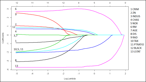
FIGURE 15-3: Visualizing the path of coefficients using various degrees of L1 regularization.
The chart represents all the coefficients by placing their standardized values on the ordinate, the vertical axis. As for as the abscissa, the scale uses a log function of lambda so that you get an idea of the small value of lambda at the leftmost side of the chart (where it’s just like a standard regression). The abscissa also shows another scale, placed in the uppermost part of the chart, that tells you how many coefficients are nonzero at that lambda value. Running from left to right, you can observe how coefficients decrease in absolute value until they become zero, telling you the story of how regularization affects a model. Naturally, if you just need to estimate a model and the coefficients for the best predictions, you need to find the correct lambda value using cross-validation:
cv <- cv.glmnet(X, y, family="gaussian", alpha=1, standardize=FALSE)coef(cv, s="lambda.min")
Learning One Example at a Time
Finding the right coefficients for a linear model is just a matter of time and memory. However, sometimes a system won’t have enough memory to store a huge dataset. In this case, you must resort to other means, such as learning from one example at a time rather than having all of them loaded into memory. The following sections help you understand the one-example-at-a-time approach to learning.
Using gradient descent
The gradient descent finds the right way to minimize the cost function one iteration at a time. After each step, it accounts for all the model’s summed errors and updates the coefficients in order to make the error even smaller during the next data iteration. The efficiency of this approach derives from considering all the examples in the sample. The drawback of this approach is that you must load all the data into memory.
Unfortunately, you can’t always store all the data in memory because some datasets are huge. In addition, learning using simple learners requires large amounts of data in order to build effective models (more data helps to correctly disambiguate multicollinearity). Getting and storing chunks of data on your hard disk is always possible, but it’s not feasible because of the need to perform matrix multiplication, which would require lots of data swapping from disk (random disk access) to select rows and columns. Scientists who have worked on the problem have found an effective solution. Instead of learning from all the data after having seen it all (which is called an iteration), the algorithm learns from one example at a time, as picked from storage using sequential access, and then goes on to learn from the next example. When the algorithm has learned all the examples, it starts again from the beginning unless some stopping criterion is met (for instance, completing a predefined number of iterations).
A data stream is the data that flows from disk, one example at a time. Streaming is the action of passing data from storage to memory. The out-of-core learning style (online learning) occurs when an algorithm learns from a stream, which is a viable learning strategy discussed at the end of Chapter 10.
Some common sources of data streams are web traffic, sensors, satellites, and surveillance recordings. An intuitive example of a stream is, for instance, the data flow produced instant by instant using a sensor, or the tweets generated by a Twitter streamline. You can also stream common data that you’re used to keeping in memory. For example, if a data matrix is too big, you can treat it as a data stream and start learning one row at a time, pulling it from a text file or a database. This kind of streaming is the online-learning style.
Understanding how SGD is different
Stochastic gradient descent (SGD) is a slight variation on the gradient descent algorithm. It provides an update procedure for estimating beta coefficients. Linear models are perfectly at ease with this approach.
In SGD, the formulation remains the same as in the standard version of gradient descent (called the batch version, in contrast to the online version), except for the update. In SGD, the update is executed a single instance at a time, allowing the algorithm to leave core data in storage and place just the single observation needed to change the coefficient vector in memory:
As with the gradient descent algorithm, the algorithm updates the coefficient, w, of feature j by subtracting the difference between the prediction and the real response. It then multiplies the difference by the value of the feature j and by a learning factor alpha (which can reduce or increase the effect of the update on the coefficient).
There are other subtle differences when using SGD rather than the gradient descent. The most important difference is the stochastic term in the name of this online learning algorithm. In fact, SGD expects an example at a time, drawn randomly from the available examples (random sampling). The problem with online learning is that example ordering changes the way the algorithm guesses beta coefficients. It’s the greediness principle discussed when dealing with decision trees (see Chapter 12): With partial optimization, one example can change the way the algorithm reaches the optimum value, creating a different set of coefficients than would have happened without that example.
As a practical example, just keep in mind that SGD can learn the order in which it sees the examples. So if the algorithm performs any kind of ordering (historical, alphabetical, or, worse, related to the response variable), it will invariably learn it. Only random sampling (meaningless ordering) allows you to obtain a reliable online model that works effectively on unseen data. When streaming data, you need to randomly reorder your data (data shuffling).
The SGD algorithm, contrary to batch learning, needs a much larger number of iterations in order to get the right global direction in spite of the contrary indications that come from single examples. In fact, the algorithm updates after each new example, and the consequent journey toward an optimum set of parameters is more erratic in comparison to an optimization made on a batch, which immediately tends to get the right direction because it’s derived from data as a whole, as shown in Figure 15-4.

FIGURE 15-4: Visualizing the different optimization paths on the same data problem.
In this case, the learning rate has even more importance because it dictates how the SGD optimization procedure can resist bad examples. In fact, if the learning rate is high, an outlying example could derail the algorithm completely, preventing it from reaching a good result. On the other hand, high learning rates help to keep the algorithm learning from examples. A good strategy is to use a flexible learning rate, that is, starting with a flexible learning rate and making it rigid as the number of examples it has seen grows.
If you think about it, as a learning strategy the flexible learning rate is similar to the one adopted by our brain: flexible and open to learn when we are children and more difficult (but not impossible) to change when we grow older. You use Python’s Scikit-learn to perform out-of-core learning because R doesn’t offer an analogous solution. Python offers two SGD implementations, one for classification problems (SGDClassifier) and one for regression problems (SGDRegressor). Both of these methods, apart from the fit method (used to fit data in memory), feature a partial_fit method that keeps previous results and learning schedule in memory, and continues learning as new examples arrive. With the partial_fit method, you can partially fit small chunks of data, or even single examples, and continue feeding the algorithm data until it finds a satisfactory result.
Both SGD classification and regression implementations in Scikit-learn feature different loss functions that you can apply to the stochastic gradient descent optimization. Only two of those functions refer to the methods dealt with in this chapter:
loss='squared_loss': Ordinary least squares (OLS) for linear regressionloss='log': Classical logistic regression
The other implementations (hinge, huber, epsilon insensitive) optimize a different kind of loss function similar to the perceptron. Chapter 17 explains them in more detail when talking about support vector machines.
To demonstrate the effectiveness of out-of-core learning, the following example sets up a brief experiment in Python using regression and squared_loss as the cost function. It demonstrates how beta coefficients change as the algorithm sees more examples. The example also passes the same data multiple times to reinforce data pattern learning. Using a test set guarantees a fair evaluation, providing measures of the capability of the algorithm to generalize to out-of-sample data.
You can freely reiterate the experiment after changing the learning parameters by modifying learning_rate and its related parameters eta0 and power_t. The learning rate determines how each observed example impacts on the optimization process, and, apart from the constant option, you can modify it using optimal (suitable for classification) and invscaling (for regression). In particular, specific parameters, eta0 and power_t, control invscaling according to the formula
When the power_t parameter is a number below one, the formula creates a gradual decay of the learning rate (t is number of examples seen), allowing it to fix what it previously learned and making it resistant to any changes induced by anomalies.
This Python example uses the Boston dataset after shuffling it and separating it into training and testing sets. The example reports the coefficients’ vector and the error measures after it sees a variable number of examples in powers of two (in order to represent learning at different steps). The experiment shows how long it takes before R2 increases and the value of coefficients stabilize.
from sklearn.cross_validation import train_test_splitfrom sklearn.linear_model import SGDRegressorX_train, X_test, y_train, y_test = train_test_split(X, y, test_size=0.33, random_state=42)SGD = SGDRegressor(penalty=None, learning_rate='invscaling', eta0=0.01, power_t=0.25)power = 17check = [2**i for i in range(power+1)]for i in range(400): for j in range(X_train.shape[0]): SGD.partial_fit(X_train[j,:].reshape(1,13), y_train[j].reshape(1,)) count = (j+1) + X_train.shape[0] * i if count in check: R2 = r2_score(y_test,SGD.predict(X_test)) print ('Example %6i R2 %0.3f coef: %s' % (count, R2, ' '.join(map(lambda x:'%0.3f' %x, SGD.coef_))))Example 131072 R2 0.724 coef: -1.098 0.891 0.374 0.849 -1.905 2.752 -0.371 -3.005 2.026 -1.396 -2.011 1.102 -3.956
No matter the amount of data, you can always fit a simple but effective linear regression model using SGD online learning capabilities.