
Chapter 9: Suggesting the Right Product by Using Matrix Factorization
Suggesting the right product is one of the most common applications of Machine Learning (ML). Every day, product recommendation systems influence our choices on the internet. Newsletters, e-commerce websites, video streaming companies, and many other services leverage this powerful ML technique to offer us meaningful suggestions about the products that we may buy or like.
In this chapter, with a hands-on and practical approach, we'll execute the main implementation steps to build a new recommendation engine using the matrix factorization algorithm.
With a gradual and incremental approach and by leveraging BigQuery ML, we'll cover the following topics:
- Introducing the business scenario
- Discovering matrix factorization
- Configuring BigQuery Flex Slots
- Exploring and preparing the dataset
- Training the matrix factorization model
- Evaluating the matrix factorization model
- Using the matrix factorization model
- Drawing business conclusions
Technical requirements
This chapter requires that you have access to a web browser and can leverage the following:
- A GCP account to access the Google Cloud Console.
- A GCP project to host the BigQuery datasets.
- BigQuery Flex slots to train matrix factorization models in BigQuery ML. The training for these kinds of algorithms is only available to flat-rate customers or customers with reservations. If you're using BigQuery with its on-demand pricing, we'll show you how to use BigQuery Flex Slots.
Now that the technical requirements are clear, let's look at our use case about the BigQuery ML matrix factorization model.
Introducing the business scenario
Imagine being a business analyst that works for the Google Merchandise e-commerce store. The website sells different Google-branded products to different users. Some of the users are registered and have their own identifier, and their clickstream activities are collected in a specific dataset.
Important note
Clickstream data is the digital footprint left by users navigating a specific website. This data typically includes the web pages they visited, the time they spent on each page, the device they used, the origin of the traffic, and other relevant information.
In this scenario, the data is collected by Google using Google Analytics 360 from the Google Merchandise e-commerce portal. This tool can be integrated with any website and allows us to gather information about the users' behavior on each page of the portal for further analysis and analytics.
The following screenshot is of the Google Merchandise Store, which sells Google-branded gadgets:
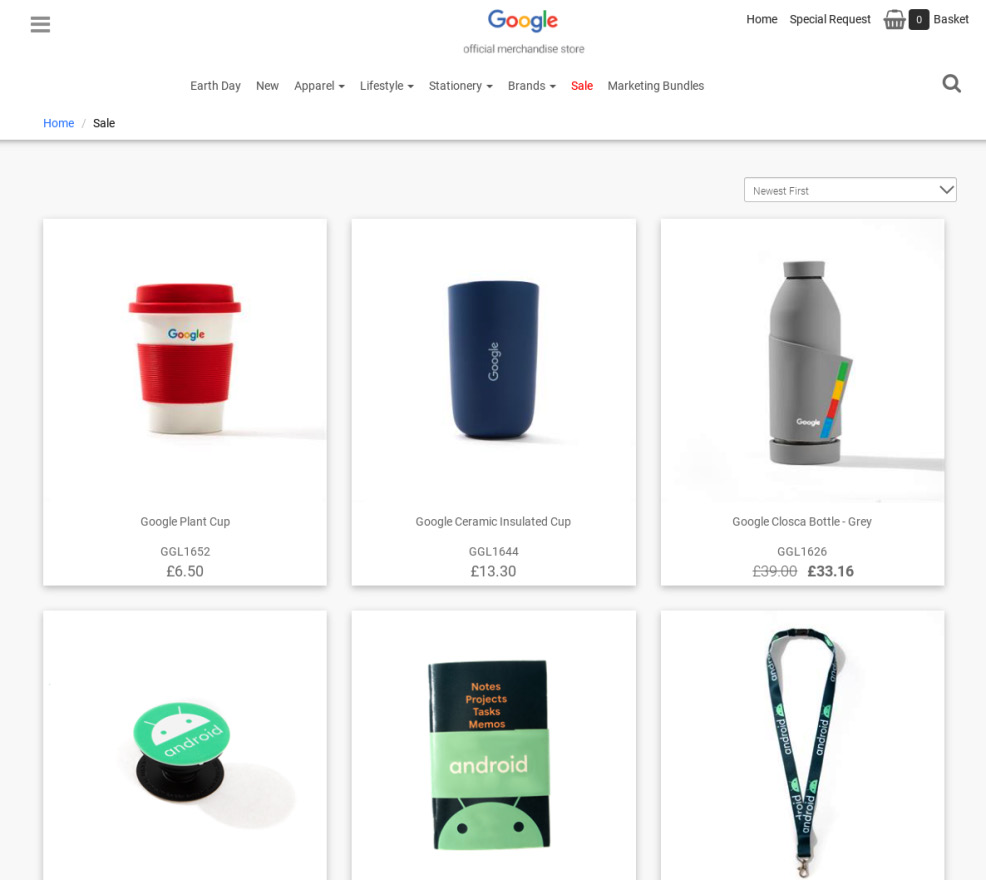
Figure 9.1 – A screenshot of the Google Merchandise Store
For our business scenario, we will imagine that our manager is asking us to build a new recommendation engine that can improve the user experience of their customers, as well as the revenues of their e-commerce sales.
Our goal is to develop a ML model that selects the right product to suggest for each customer who's registered on the website. To achieve this goal, we will use the clickstream data from the Google Merchandise Store that has already been collected and published in a BigQuery public dataset.
As business analysts, our job is to analyze the data, build an effective recommendation engine, and use it on the existing data to provide meaningful information to the marketing team.
Now that we've explained and understood the business scenario, let's take a look at the ML technique that we will use to build a recommendation engine for our e-commerce portal.
Discovering matrix factorization
In this section, we'll learn what matrix factorization is, and how it can be used to build recommendation engines.
Matrix factorization represents a class of algorithms usually used to build recommendation engines. These algorithms are built on matrices that represent the interactions between users and items. In these kinds of matrices, the following occurs:
- Each user or customer is represented as a row.
- Each item or product corresponds to a column of the matrix.
- Each cell of the matrix is filled with a numeric value: the feedback.
This feedback represents a rating that a specific user has given to a specific item.
In the following screenshot, we can see an example of a matrix where the rows are the customers of a video streaming service and the columns are the films offered by the platform. Some of the cells contain a rating that ranges from 1 to 5:

Figure 9.2 – Representation of a recommendation matrix
In this example, we can say that User 1 has expressed an average rating for the film The Shining, but disliked Titanic. On the other hand, User 4 assigned the maximum rating to Titanic, but didn't rate the other films.
According to different business scenarios, this feedback can be considered explicit or implicit:
- Explicit feedback is available when the user voluntarily rates a specific item, such as on a review website.
- If explicit feedback is not available, implicit feedback can be calculated and inferred by the developer of the recommendation system. For example, if a customer has bought a product, we can assume they would give positive feedback for that item.
Often, in e-commerce data, feedback is not explicitly given by the users but can be extracted from other information that's collected in the process, such as the number of clicks, the time spent on a specific page, or the quantity of a specific product bought by the user.
Matrix factorization algorithms are widely used in real-life scenarios. Some examples are as follows:
- The suggested books that we see in an online bookshop.
- The recommended TV series that we can see on video streaming services.
- The posts that are highlighted in our social media feeds.
- The products suggested by internet advertising systems.
In this section, we learned about the basics of matrix factorization. Now, let's configure BigQuery Flex Slots.
Configuring BigQuery Flex Slots
In this chapter, we'll understand how to configure BigQuery Flex Slots to train our ML model.
A BigQuery Slot is a unit of BigQuery analytics capacity that's used to execute SQL queries and train BigQuery ML models. One BigQuery slot represents the compute capacity of a Virtual Compute Processing Unit (VCPU).
Flex Slots allow us to buy BigQuery analytics capacity for short periods. They are usually used to quickly satisfy sudden demands for resources with a minimum duration of 60 seconds.
Enabling Flex Slots is mandatory to train a matrix factorization model; otherwise, BigQuery will return an error during the training stage.
Let's see how we can enable BigQuery Flex Slots if we're using an on-demand plan:
- If you haven't enabled BigQuery Reservations yet, we need to access Reservations from the BigQuery menu on the left:
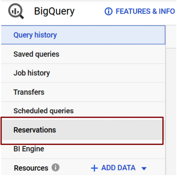
Figure 9.3 – Accessing Reservations from the BigQuery navigation menu
- Click on the BUY SLOTS button to initialize the buying process for BigQuery Flex Slots:
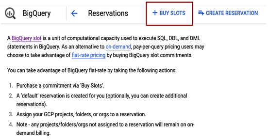
Figure 9.4 – Screenshot of the Reservations page
- Choose the minimum number of Flex Slots to buy; that is, 100. Then, click on the NEXT button:

Figure 9.5 – BigQuery Buy Slots process
- Confirm your choice by writing CONFIRM in the confirmation text box and clicking on the blue PURCHASE button:

Figure 9.6 – Confirming your BigQuery Slots purchase
- Once the purchase has been confirmed, you can switch to the ASSIGNMENTS tab to assign the reservation that you've just bought.
- On the ASSIGNMENTS tab, select your GCP project in the first combo box and the reservation of Flex Slots in the second. After that, click the CREATE button to finalize your configuration:

Figure 9.7 – Assigning BigQuery slots
- When the assignment is complete, we can go back to the BigQuery home page.
Important note
Warning: Remember to deactivate the reservation of BigQuery slots at the end of this use case. Every BigQuery slot costs $0.04 per hour. Forgetting to disable this reservation will generate unexpected billing for your GCP project.
In this section, we learned how to buy BigQuery Flex Slots so that we can use matrix factorization. Now, we will focus on the data exploration and preparation steps.
Exploring and preparing the dataset
In this section, we'll analyze the data we'll use to train our BigQuery ML model and apply the data preparation steps.
Let's start by getting a clear understanding of the Google Analytics data that is available in the BigQuery public dataset so that we can build our recommendation system.
Understanding the data
In this section, we'll import the necessary data and then understand the most relevant fields of the dataset that will be used to train the BigQuery ML model.
Before we start developing the ML model, we'll look at the dataset and its schema. To start exploring the dataset, we need to do the following:
- Log into our Google Cloud Console and access the BigQuery user interface from the navigation menu.
- Create a new dataset under the project that we created in Chapter 2, Setting Up Your GCP and BigQuery Environment. For this use case, we'll create the 09_recommendation_engine dataset with the default options.
- After that, we need to open the bigquery-public-data GCP project, which hosts the BigQuery public datasets, and browse the datasets until we find google_analytics_sample.
- The BigQuery public dataset contains multiple tables that host the Google Analytics sample data. Each table presents a different suffix according to the year and the month that it refers to:

Figure 9.8 – The Google Analytics sample dataset containing the ga_sessions tables
We'll use the ga_sessions tables to build our matrix factorization model.
Tip
The ga_sessions table is not well described, but if we need further information about this dataset, we can leverage the examples available in the BigQuery documentation at https://support.google.com/analytics/answer/4419694?hl=en.
- To simplify the data access process, let's create a single table that unifies all the tables with different suffixes. Let's execute the following SQL statement:
CREATE OR REPLACE TABLE `09_recommendation_engine.all_ga_sessions` AS
SELECT * FROM `bigquery-public-data.google_analytics_sample.ga_sessions_*`;
The query creates a new table called all_ga_sessions in our 09_recommendation_engine dataset. This table stores all the data that comes from the different ga_sessions tables into a unique structure. To unify all the records, we've used the wildcard character, *.
Tip
Wildcards are useful when a dataset contains multiple tables with similar names and compatible schemas. In this case, we're collecting all the data from the multiple ga_sessions_* tables and placing them in our new structure, all_ga_sessions.
- Now, we can simply query all_ga_sessions to get a preview of the schema:
SELECT * FROM `09_recommendation_engine.all_ga_sessions`
TABLESAMPLE SYSTEM (10 PERCENT);
The results of the query point out that the schema of the table is quite complex and contains multiple nested fields. Fortunately, for our purposes, we will only focus on some of them:
fullVisitorID represents the identifier of each registered user that is browsing Google's website.
productSku is the product code that identifies a specific product in Google's catalog. Some examples of products are mugs, T-shirts, bags, and socks.
The action_type column is the action that a user has performed during a web session. If this field is equal to 6, the row represents a specific product being purchased by a customer.
Now that we've discovered which columns will be used for our ML model, it's time to prepare our training dataset.
Creating the training dataset
In this section, we'll create the tables that will host the training data of our BigQuery ML model.
To train our model, we'll create a table that will host all the purchases that have been made by the registered customers on the website.
Let's create the product_purchases table, which contains three fields:
- The code of each user: fullVisitorId
- The identifier of the purchased product: purchased_product_id
- The quantity field, which specifies the product that's been bought by the customer
Execute the following SQL statement to create the table:
CREATE OR REPLACE TABLE `09_recommendation_engine.product_purchases` AS
SELECT fullVisitorId,
hits_product.productSKU AS purchased_product_id,
COUNT(hits_product.productSKU) AS quantity
FROM
`09_recommendation_engine.all_ga_sessions`,
UNNEST(hits) AS hits,
UNNEST(hits.product) AS hits_product
WHERE fullVisitorId IN (
SELECT fullVisitorId
FROM
`09_recommendation_engine.all_ga_sessions`,
UNNEST(hits) AS hits
WHERE
hits.eCommerceAction.action_type = '6'
GROUP BY fullVisitorId
)
GROUP BY fullVisitorId, purchased_product_id;
The most internal query extracts all the customers identified by fullVisitorId from the all_ga_sessions table that have at least bought a product on the e-commerce portal. To identify these purchases, we've added a WHERE clause to hits.eCommerceAction.action_type = '6'. To get distinct values of fullVisitorId, the query leverages the GROUP BY fullVisitorId clause.
In the FROM clause of the nested query, we're using the UNNEST function to extract the nested fields present in the original table and access them.
Important note
UNNEST is a function that's used to convert an array into a set of multiple rows. It takes an array as input and returns a table with a single row for each item in the array.
In the most external query, we simply extract the three fields that are relevant to our use case: fullVisitorId, purchased_product_id, and our total quantity. This last measure is obtained by using the SUM operator on all the transactions being performed by a specific user to buy a specific product.
Now that we've created the table that our recommendation engine will be trained on, let's create the BigQuery ML model.
Training the matrix factorization model
In this section, we'll train the BigQuery ML matrix factorization model in order to build a recommendation system with the e-commerce data that we've already prepared.
Let's start training the purchase_recommender ML model by executing the following SQL statement:
CREATE OR REPLACE MODEL `09_recommendation_engine.purchase_recommender`
OPTIONS(model_type='matrix_factorization',
user_col='fullVisitorID',
item_col='purchased_product_id',
rating_col='quantity',
feedback_type='implicit'
)
AS
SELECT fullVisitorID, purchased_product_id, quantity
FROM `09_recommendation_engine.product_purchases`;
The first few lines of the query are composed of the CREATE OR REPLACE MODEL keywords, followed by the identifier of the new ML model, `09_recommendation_engine.purchase_recommender`, and OPTIONS.
Now, let's focus on the OPTIONS values that we've used to train our BigQuery ML model:
- The model type is 'matrix_factorization'. This option describes the algorithm that we're using to train our recommendation model.
- The user_col='fullVisitorID' option specifies which column represents the users of the recommendation engine. In our case, we're using the fullVisitorID field, which is assigned to the registered customers of the e-commerce portal.
- With the item_col='purchased_product_id' option, we're using the code of each product that's been purchased by our customers to identify each item in our model.
- Since we don't have an explicit rating for our products, we'll choose feedback_type='implicit' and use the purchased quantity value as the rating for our recommendation engine. In this case, we're assuming that if a user has bought large quantities of a product, they're interested and satisfied with the product.
After about 7 minutes, the matrix factorization model will be trained, and we can move on to the next stage: the evaluation phase.
Evaluating the matrix factorization model
In this section, we'll evaluate the performances of the matrix factorization model that we trained in the previous section.
The evaluation stage of a matrix factorization model can be performed using the ML.EVALUATE BigQuery ML function or through the BigQuery UI.
Let's execute the following query to extract all the evaluation parameters that characterize the recommendation model that we've just trained:
SELECT
*
FROM
ML.EVALUATE(MODEL `09_recommendation_engine.recommender`,
(
SELECT * FROM `09_recommendation_engine.product_visits`));
The result of this query is shown in the following screenshot:

Figure 9.9 – The record that's been extracted from the evaluation of the matrix factorization model
The same information can be accessed by selecting the ML model from the BigQuery navigation menu and then accessing the Evaluation tab.
In the following screenshot, you can see the evaluation metrics of the BigQuery ML model:
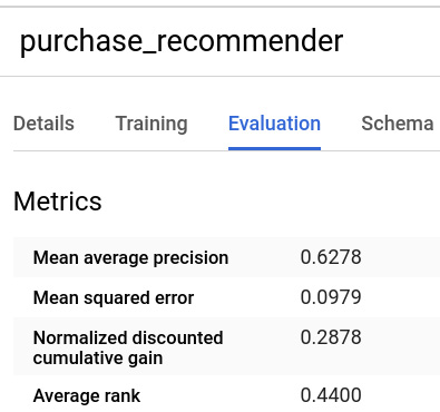
Figure 9.10 – The Evaluation tab of the matrix factorization model
Since the value of Mean squared error is very low, we can be satisfied with the results that have been achieved by our matrix factorization model.
In this section, we learned how to access the performance indicators of our recommendation model. Now, let's use the recommendation model to find the best products to suggest to our customers.
Using the matrix factorization model
In this section, we'll test the matrix factorization model to get the recommended products for the users of our website.
To use our BigQuery ML model, we'll use the ML.RECOMMEND function while specifying the parameters for our prediction.
The recommendation engine does not need to take any additional input parameters besides the model itself. If the model has one input column, the model will only return the recommendations for the rows in the input. If no input values are provided, the model will apply the prediction for each combination of users and items in the original dataset.
ML.RECOMMEND returns three columns:
- A column that represents the user. In our implementation, this is identified by the fullVisitorID column.
- A field dedicated to the item that is recommended to a specific user. In our case, this is represented by the purchased_product_id column.
- A third column that represents the predicted rating in the case of an explicit matrix factorization model. If the model is implicit, as in our case, the field stores the predicted confidence of the recommendation.
Let's execute the following query to materialize a table that contains all the recommendations that have been generated by our matrix factorization model:
CREATE OR REPLACE TABLE `09_recommendation_engine.product_recommendations` AS
SELECT
DISTINCT fullVisitorID, purchased_product_id, predicted_quantity_confidence
FROM
ML.RECOMMEND(MODEL`09_recommendation_engine.purchase_recommender`,
(
SELECT
fullVisitorID
FROM
`09_recommendation_engine.product_purchases` ));
The query creates a new table called product_recommendations that stores the DISTINCT couples of users and items. In our case, the couples are composed of the fullVisitorID and purchased_product_id columns.
For each couple, the ML.RECOMMEND function also returns a predicted confidence that expresses the probability that a specific user has interest in a product in the e-commerce catalog.
Now that we have the output of our recommendation engine, let's learn how to use this data from a business perspective.
Drawing business conclusions
Now that we've applied our BigQuery ML model, let's learn how the generated results can be used from a business perspective to improve the effectiveness of our sales strategy.
From the product_recommendations table, we can extract relevant information that we can use to improve our marketing campaigns or advertising strategy, and then target the users with higher propensity to buy a specific product.
For example, by executing the following query, we can extract the first 100 users with the highest propensity to buy a specific product from our e-commerce portal:
SELECT *
FROM
`09_recommendation_engine.product_recommendations`
ORDER BY predicted_quantity_confidence DESC
LIMIT 100;
Executing this SQL statement returns the following result:
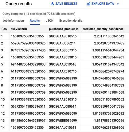
Figure 9.11 – The customers with the highest propensity to buy a specific product
The list that we've just extracted can be sent to our marketing office to create tailored marketing campaigns. Alternatively, it can be used in our e-commerce portal to recommend the most interesting products for a specific registered customer.
Summary
In this chapter, we built a recommendation engine based on the matrix factorization algorithm. After we introduced the business scenario, we discovered what matrix factorization is and the difference between explicit and implicit models. Before diving into data exploration, we enabled BigQuery Flex Slots, which are necessary to train this category of ML algorithms.
Then, we applied some analyses and data preparation steps to the sample data collected by Google from the Google Merchandise e-commerce portal. Here, we've focused on the fields that were actually required to build our BigQuery ML model.
Next, we created our training table, which includes the purchases that were made by each user, along with the related quantity for each product.
After that, we trained our matrix factorization model on the data that we'd prepared. When the model was trained, we evaluated its key performance indicators using SQL code and the BigQuery UI.
Finally, we generated some recommendations using our new matrix factorization model and extracted a list of 100 customers that can be targeted with high propensity to buy a set of products.
In the next chapter, we'll introduce the XGBoost algorithm for predicting binary values.
Further resources
- Google Analytics 360 public dataset: https://console.cloud.google.com/marketplace/product/obfuscated-ga360-data/obfuscated-ga360-data
- BigQuery ML create model: https://cloud.google.com/bigquery-ml/docs/reference/standard-sql/bigqueryml-syntax-create
- BigQuery ML evaluate model: https://cloud.google.com/bigquery-ml/docs/reference/standard-sql/bigqueryml-syntax-evaluate
- BigQuery ML RECOMMEND: https://cloud.google.com/bigquery-ml/docs/reference/standard-sql/bigqueryml-syntax-recommend
- BigQuery ML explicit matrix factorization example: https://cloud.google.com/bigquery-ml/docs/bigqueryml-mf-explicit-tutorial
- BigQuery ML implicit matrix factorization example: https://cloud.google.com/bigquery-ml/docs/bigqueryml-mf-implicit-tutorial#implicit-model