
When a meteorologist provides a weather forecast, precipitation is typically described with phrases like "70 percent chance of rain." Such forecasts are known as probability of precipitation reports. Have you ever considered how they are calculated? It is a puzzling question because in reality, either it will rain or not.
Weather estimates are based on probabilistic methods, which are those concerned with describing uncertainty. They use data on past events to extrapolate future events. In the case of the weather, the chance of rain describes the proportion of prior days with similar atmospheric conditions in which precipitation occurred. A 70 percent chance of rain implies that in seven out of 10 past cases with similar conditions, precipitation occurred somewhere in the area.
This chapter covers the Naive Bayes algorithm, which uses probabilities in much the same way as a weather forecast. While studying this method, you will learn:
- Basic principles of probability
- The specialized methods and data structures needed to analyze text data with R
- How to employ Naive Bayes to build an SMS junk message filter
If you've taken a statistics class before, some of the material in this chapter may be a review. Even so, it may be helpful to refresh your knowledge of probability, as these principles are the basis of how Naive Bayes got such a strange name.
The basic statistical ideas necessary to understand the Naive Bayes algorithm have existed for centuries. The technique descended from the work of the 18th century mathematician Thomas Bayes, who developed foundational principles for describing the probability of events and how probabilities should be revised in light of additional information. These principles formed the foundation for what are now known as Bayesian methods.
We will cover these methods in greater detail later on. For now, it suffices to say that a probability is a number between zero and one (that is, from zero to 100 percent), which captures the chance that an event will occur in light of the available evidence. The lower the probability, the less likely the event is to occur. A probability of zero indicates that the event will definitely not occur, while a probability of one indicates that the event will occur with absolute certainty.
Classifiers based on Bayesian methods utilize training data to calculate the probability of each outcome based on the evidence provided by feature values. When the classifier is later applied to unlabeled data, it uses these calculated probabilities to predict the most likely class for the new example. It's a simple idea, but it results in a method that can have results on a par with more sophisticated algorithms. In fact, Bayesian classifiers have been used for:
- Text classification, such as junk email (spam) filtering
- Intrusion or anomaly detection in computer networks
- Diagnosing medical conditions given a set of observed symptoms
Typically, Bayesian classifiers are best applied to problems in which the information from numerous attributes should be considered simultaneously in order to estimate the overall probability of an outcome. While many machine learning algorithms ignore features that have weak effects, Bayesian methods utilize all available evidence to subtly change the predictions. This implies that even if a large number of features have relatively minor effects, their combined impact in a Bayesian model could be quite large.
Before jumping into the Naive Bayes algorithm, it's worth spending some time defining the concepts that are used across Bayesian methods. Summarized in a single sentence, Bayesian probability theory is rooted in the idea that the estimated likelihood of an event, or potential outcome, should be based on the evidence at hand across multiple trials, or opportunities for the event to occur.
The following table illustrates events and trials for several real-world outcomes:
|
Event |
Trial |
|---|---|
|
Heads result |
Coin flip |
|
Rainy weather |
A single day |
|
Message is spam |
Incoming email message |
|
Candidate becomes president |
Presidential election |
|
Win the lottery |
Lottery ticket |
Bayesian methods provide insights into how the probability of these events can be estimated from observed data. To see how, we'll need to formalize our understanding of probability.
The probability of an event is estimated from observed data by dividing the number of trials in which the event occurred by the total number of trials. For instance, if it rained three out of 10 days with similar conditions as today, the probability of rain today can be estimated as 3 / 10 = 0.30 or 30 percent. Similarly, if 10 out of 50 prior email messages were spam, then the probability of any incoming message being spam can be estimated as 10 / 50 = 0.20 or 20 percent.
To denote these probabilities, we use notation in the form P(A), which signifies the probability of event A. For example, P(rain) = 0.30 and P(spam) = 0.20.
The probability of all possible outcomes of a trial must always sum to one, because a trial always results in some outcome happening. Thus, if the trial has two outcomes that cannot occur simultaneously, such as rainy versus sunny, or spam versus ham (not spam), then knowing the probability of either outcome reveals the probability of the other. For example, given the value P(spam) = 0.20, we can calculate P(ham) = 1 – 0.20 = 0.80. This works because spam and ham are mutually exclusive and exhaustive events, which implies that they cannot occur at the same time and are the only possible outcomes.
Now, because an event cannot happen and not happen simultaneously, an event is always mutually exclusive and exhaustive with its complement, or the event comprising the outcomes in which the event of interest does not happen. The complement of event A is typically denoted Ac or A'. Additionally, the shorthand notation P(¬A) can be used to denote the probability of event A not occurring, as in P(¬spam) = 0.80. This notation is equivalent to P(Ac).
To illustrate events and their complements, it is often helpful to imagine a two-dimensional space that is partitioned into probabilities for each event. In the following diagram, the rectangle represents the possible outcomes for an email message. The circle represents the 20 percent probability that the message is spam. The remaining 80 percent represents the complement P(¬spam), or the messages that are not spam:
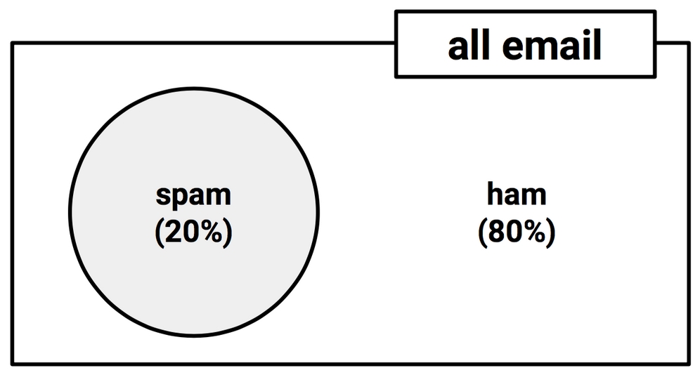
Figure 4.1: The probability space of all email can be visualized as partitions of spam and ham
Often, we are interested in monitoring several non-mutually exclusive events for the same trial. If certain events occur concurrently with the event of interest, we may be able to use them to make predictions. Consider, for instance, a second event based on the outcome that an email message contains the word "Viagra." The preceding diagram, updated for this second event, might appear as shown in the following diagram:
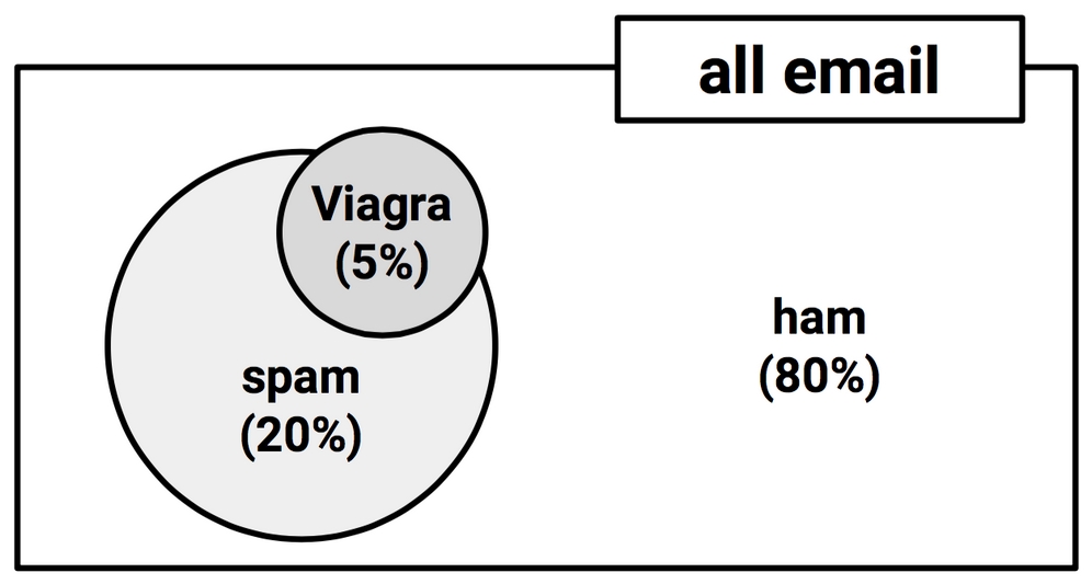
Figure 4.2: Non-mutually exclusive events are depicted as overlapping partitions
Notice in the diagram that the Viagra circle does not completely fill the spam circle, nor is it completely contained by the spam circle. This implies that not all spam messages contain the word "Viagra" and not every email with the word "Viagra" is spam. However, because this word appears very little outside spam, its presence in a new incoming message would be strong evidence that the message is spam.
To zoom in for a closer look at the overlap between these circles, we'll employ a visualization known as a Venn diagram. First used in the late 19th century by mathematician John Venn, the diagram uses circles to illustrate the overlap between sets of items. As is the case here, in most Venn diagrams, the size of the circles and the degree of the overlap is not meaningful.
Instead, it is used as a reminder to allocate probability to all combinations of events. A Venn diagram for spam and Viagra might be depicted as follows:
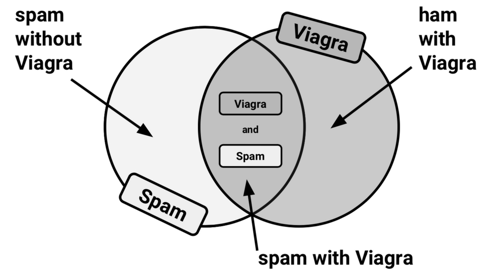
Figure 4.3: A Venn diagram illustrates the overlap of the spam and Viagra events
We know that 20 percent of all messages were spam (the left circle), and 5 percent of all messages contained the word "Viagra" (the right circle). We would like to quantify the degree of overlap between these two proportions. In other words, we hope to estimate the probability that both P(spam) and P(Viagra) occur, which can be written as P(spam ∩ Viagra). The upside-down "U" symbol signifies the intersection of the two events; the notation A ∩ B refers to the event in which both A and B occur.
Calculating P(spam ∩ Viagra) depends on the joint probability of the two events, or how the probability of one event is related to the probability of the other. If the two events are totally unrelated, they are called independent events. This is not to say that independent events cannot occur at the same time; event independence simply implies that knowing the outcome of one event does not provide any information about the outcome of the other. For instance, the outcome of a heads result on a coin flip is independent from whether the weather is rainy or sunny on any given day.
If all events were independent, it would be impossible to predict one event by observing another. In other words, dependent events are the basis of predictive modeling. Just as the presence of clouds is predictive of a rainy day, the appearance of the word "Viagra" is predictive of a spam email.

Figure 4.4: Dependent events are required for machines to learn to identify useful patterns
Calculating the probability of dependent events is a bit more complex than for independent events. If P(spam) and P(Viagra) were independent, we could easily calculate P(spam ∩ Viagra), the probability of both events happening at the same time. Because 20 percent of all messages are spam, and 5 percent of all emails contain the word "Viagra," we could assume that 1 percent of all messages are spam with the term "Viagra." This is because 0.05 * 0.20 = 0.01. More generally, for independent events A and B, the probability of both happening can be computed as P(A ∩ B) = P(A) * P(B).
That said, we know that P(spam) and P(Viagra) are likely to be highly dependent, which means that this calculation is incorrect. To obtain a more reasonable estimate, we need to use a more careful formulation of the relationship between these two events, which is based on more advanced Bayesian methods.
The relationships between dependent events can be described using Bayes' theorem, which provides a way of thinking about how to revise an estimate of the probability of one event in light of the evidence provided by another. One formulation is as follows:
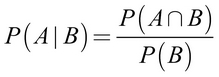
The notation P(A|B) is read as the probability of event A given that event B occurred. This is known as conditional probability, since the probability of A is dependent (that is, conditional) on what happened with event B. Bayes' theorem tells us that our estimate of P(A|B) should be based on P(A ∩ B), a measure of how often A and B are observed to occur together, and P(B), a measure of how often B is observed to occur in general.
Bayes' theorem states that the best estimate of P(A|B) is the proportion of trials in which A occurred with B, out of all the trials in which B occurred. This implies that the probability of event A is higher if A and B often occur together each time B is observed. Note that this formula adjusts P(A ∩ B) for the probability of B occurring. If B is extremely rare, P(B) and P(A ∩ B) will always be small; however, if A and B almost always happen together, P(A|B) will be high regardless of the probability of B.
By definition, P(A ∩ B) = P(A|B) * P(B), a fact which can be easily derived by applying a bit of algebra to the previous formula. Rearranging this formula once more with the knowledge that P(A ∩ B) = P(B ∩ A) results in the conclusion that P(A ∩ B) = P(B|A) * P(A), which we can then use in the following formulation of Bayes' theorem:
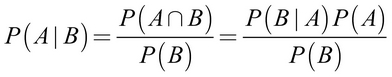
In fact, this is the traditional formulation of Bayes' theorem, for reasons that will become clear as we apply it to machine learning. First, to better understand how Bayes' theorem works in practice, let's revisit our hypothetical spam filter.
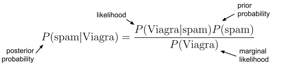
Without knowledge of an incoming message's content, the best estimate of its spam status would be P(spam), the probability that any prior message was spam. This estimate is known as the prior probability. We found this previously to be 20 percent.
Suppose that you obtained additional evidence by looking more carefully at the set of previously received messages and examining the frequency that the term "Viagra" appeared. The probability that the word "Viagra" was used in previous spam messages, or P(Viagra|spam), is called the likelihood. The probability that "Viagra" appeared in any message at all, or P(Viagra), is known as the marginal likelihood.
By applying Bayes' theorem to this evidence, we can compute a posterior probability that measures how likely a message is to be spam. If the posterior probability is greater than 50 percent, the message is more likely to be spam than ham, and it should perhaps be filtered. The following formula shows how Bayes' theorem is applied to the evidence provided by previous email messages:
To calculate the components of Bayes' theorem, it helps to construct a frequency table (shown on the left in the following diagram) that records the number of times "Viagra" appeared in spam and ham messages. Just like a two-way cross-tabulation, one dimension of the table indicates levels of the class variable (spam or ham), while the other dimension indicates levels for features (Viagra: yes or no). The cells then indicate the number of instances that have the particular combination of class value and feature value.
The frequency table can then be used to construct a likelihood table, as shown on the right in the following diagram. The rows of the likelihood table indicate the conditional probabilities for "Viagra" (yes/no), given that an email was either spam or ham.
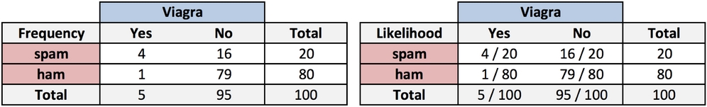
Figure 4.5: Frequency and likelihood tables are the basis for computing the posterior probability of spam
The likelihood table reveals that P(Viagra=Yes|spam) = 4 / 20 = 0.20, indicating that there is a 20 percent probability a message contains the term "Viagra" given that the message is spam. Additionally, since P(A ∩ B) = P(B|A) * P(A), we can calculate P(spam ∩ Viagra) as P(Viagra|spam) * P(spam) = (4 / 20) * (20 / 100) = 0.04. The same result can be found in the frequency table, which notes that four out of 100 messages were spam with the term "Viagra." Either way, this is four times greater than the previous estimate of 0.01 we calculated as P(A ∩ B) = P(A) * P(B) under the false assumption of independence. This, of course, illustrates the importance of Bayes' theorem for estimating joint probability.
To compute the posterior probability, P(spam|Viagra), we simply take P(Viagra|spam) * P(spam) / P(Viagra), or (4 / 20) * (20 / 100) / (5 / 100) = 0.80. Therefore, the probability is 80 percent that a message is spam, given that it contains the word "Viagra." In light of this result, any message containing this term should probably be filtered.
This is very much how commercial spam filters work, although they consider a much larger number of words simultaneously when computing the frequency and likelihood tables. In the next section, we'll see how this method is put to use when additional features are involved.
The Naive Bayes algorithm defines a simple method to apply Bayes' theorem to classification problems. Although it is not the only machine learning method that utilizes Bayesian methods, it is the most common. It grew in popularity due to its successes in text classification, where it was once the de facto standard. The strengths and weaknesses of this algorithm are as follows:
|
Strengths |
Weaknesses |
|---|---|
|
|
The Naive Bayes algorithm is named as such because it makes some "naive" assumptions about the data. In particular, Naive Bayes assumes that all of the features in the dataset are equally important and independent. These assumptions are rarely true in most real-world applications.
For example, if you were attempting to identify spam by monitoring email messages, it is almost certainly true that some features will be more important than others. For example, the email sender may be a more important indicator of spam than the message text. Additionally, the words in the message body are not independent from one another, since the appearance of some words is a very good indication that other words are also likely to appear. A message with the word "Viagra" will probably also contain the words "prescription" or "drugs."
However, in most cases, even when these assumptions are violated, Naive Bayes still performs fairly well. This is true even in circumstances where strong dependencies are found among the features. Due to the algorithm's versatility and accuracy across many types of conditions, particularly with smaller training datasets, Naive Bayes is often a reasonable baseline candidate for classification learning tasks.
Note
The exact reason why Naive Bayes works well in spite of its faulty assumptions has been the subject of much speculation. One explanation is that it is not important to obtain a precise estimate of probability so long as the predictions are accurate. For instance, if a spam filter correctly identifies spam, does it matter whether it was 51 percent or 99 percent confident in its prediction? For one discussion of this topic, refer to On the Optimality of the Simple Bayesian Classifier under Zero-One Loss, Domingos P and Pazzani M, Machine Learning, 1997, Vol. 29, pp. 103-130.
Let's extend our spam filter by adding a few additional terms to be monitored in addition to the term "Viagra": "money," "groceries," and "unsubscribe." The Naive Bayes learner is trained by constructing a likelihood table for the appearance of these four words (labeled W1, W2, W3, and W4), as shown in the following diagram for 100 emails:

Figure 4.6: An expanded table adds likelihoods for additional terms in spam and ham messages
As new messages are received, we need to calculate the posterior probability to determine whether they are more likely spam or ham, given the likelihood of the words being found in the message text. For example, suppose that a message contains the terms "Viagra" and "unsubscribe" but does not contain either "money" or "groceries."
Using Bayes' theorem, we can define the problem as shown in the following formula. This computes the probability that a message is spam, given that Viagra = Yes, Money = No, Groceries = No, and Unsubscribe = Yes:
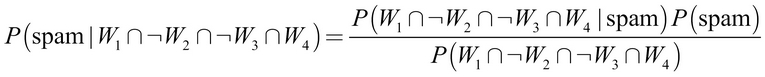
For a number of reasons, this formula is computationally difficult to solve. As additional features are added, tremendous amounts of memory are needed to store probabilities for all of the possible intersecting events. Imagine the complexity of a Venn diagram for the events for four words, let alone for hundreds or more. Many of these potential intersections will never have been observed in past data, which would lead to a joint probability of zero and problems that will become clear later.
The computation becomes more reasonable if we exploit the fact that Naive Bayes makes the naive assumption of independence among events. Specifically, it assumes class-conditional independence, which means that events are independent so long as they are conditioned on the same class value. The conditional independence assumption allows us to use the probability rule for independent events, which states that P(A ∩ B) = P(A) * P(B). This simplifies the numerator by allowing us to multiply the individual conditional probabilities rather than computing a complex conditional joint probability.
Lastly, because the denominator does not depend on the target class (spam or ham), it is treated as a constant value and can be ignored for the time being. This means that the conditional probability of spam can be expressed as:
And the probability that the message is ham can be expressed as:
Note that the equals symbol has been replaced by the proportional-to symbol (similar to a sideways, open-ended "8") to indicate the fact that the denominator has been omitted.
Using the values in the likelihood table, we can start filling numbers in these equations. The overall likelihood of spam is then:
(4 / 20) * (10 / 20) * (20 / 20) * (12 / 20) * (20 / 100) = 0.012
While the likelihood of ham is:
(1 / 80) * (66 / 80) * (71 / 80) * (23 / 80) * (80 / 100) = 0.002
Because 0.012 / 0.002 = 6, we can say that this message is six times more likely to be spam than ham. However, to convert these numbers to probabilities, we need one last step to reintroduce the denominator that had been excluded. Essentially, we must re-scale the likelihood of each outcome by dividing it by the total likelihood across all possible outcomes.
In this way, the probability of spam is equal to the likelihood that the message is spam divided by the likelihood that the message is either spam or ham:
0.012 / (0.012 + 0.002) = 0.857
Similarly, the probability of ham is equal to the likelihood that the message is ham divided by the likelihood that the message is either spam or ham:
0.002 / (0.012 + 0.002) = 0.143
Given the pattern of words found in this message, we expect that the message is spam with 85.7 percent probability, and ham with 14.3 percent probability. Because these are mutually exclusive and exhaustive events, the probabilities sum up to one.
The Naive Bayes classification algorithm used in the preceding example can be summarized by the following formula. The probability of level L for class C, given the evidence provided by features F1 through Fn, is equal to the product of the probabilities of each piece of evidence conditioned on the class level, the prior probability of the class level, and a scaling factor 1 / Z, which converts the likelihood values to probabilities. This is formulated as:
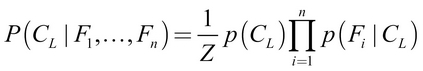
Although this equation seems intimidating, as the spam filtering example illustrated, the series of steps is fairly straightforward. Begin by building a frequency table, use this to build a likelihood table, and multiply out the conditional probabilities with the "naive" assumption of independence. Finally, divide by the total likelihood to transform each class likelihood into a probability. After attempting this calculation a few times by hand, it will become second nature.
Before we employ Naive Bayes on more complex problems, there are some nuances to consider. Suppose we received another message, this time containing all four terms: "Viagra," "groceries," "money," and "unsubscribe." Using the Naive Bayes algorithm as before, we can compute the likelihood of spam as:
(4 / 20) * (10 / 20) * (0 / 20) * (12 / 20) * (20 / 100) = 0
And the likelihood of ham is:
(1 / 80) * (14 / 80) * (8 / 80) * (23 / 80) * (80 / 100) = 0.00005
Therefore, the probability of spam is:
0 / (0 + 0.00005) = 0
And the probability of ham is:
0.00005 / (0 + 0. 0.00005) = 1
These results suggest that the message is spam with zero percent probability and ham with 100 percent probability. Does this prediction make sense? Probably not. The message contains several words usually associated with spam, including "Viagra," which is rarely used in legitimate messages. It is therefore very likely that the message has been incorrectly classified.
This problem arises if an event never occurs for one or more levels of the class and therefore their joint probability is zero. For instance, the term "groceries" had never previously appeared in a spam message. Consequently, P(spam|groceries) = 0%.
Now, because probabilities in the Naive Bayes formula are multiplied in a chain, this zero percent value causes the posterior probability of spam to be zero, giving the word "groceries" the ability to effectively nullify and overrule all of the other evidence. Even if the email was otherwise overwhelmingly expected to be spam, the absence of the word "groceries" in spam will always veto the other evidence and result in the probability of spam being zero.
A solution to this problem involves using something called the Laplace estimator, which is named after the French mathematician Pierre-Simon Laplace. The Laplace estimator adds a small number to each of the counts in the frequency table, which ensures that each feature has a non-zero probability of occurring with each class. Typically, the Laplace estimator is set to one, which ensures that each class-feature combination is found in the data at least once.
Tip
The Laplace estimator can be set to any value and does not necessarily even have to be the same for each of the features. If you were a devoted Bayesian, you could use a Laplace estimator to reflect a presumed prior probability of how the feature relates to the class. In practice, given a large enough training dataset, this is excessive. Consequently, the value of one is almost always used.
Let's see how this affects our prediction for this message. Using a Laplace value of one, we add one to each numerator in the likelihood function. Then, we need to add four to each conditional probability denominator to compensate for the four additional values added to the numerator. The likelihood of spam is therefore:
(5 / 24) * (11 / 24) * (1 / 24) * (13 / 24) * (20 / 100) = 0.0004
And the likelihood of ham is:
(2 / 84) * (15 / 84) * (9 / 84) * (24 / 84) * (80 / 100) = 0.0001
By computing 0.0004 / (0.0004 + 0.0001), we find that the probability of spam is 80 percent and therefore the probability of ham is about 20 percent. This is a more plausible result than the P(spam) = 0 computed when the term "groceries" alone determined the result.
Tip
Although the Laplace estimator was added to the numerator and denominator of the likelihoods, it was not added to the prior probabilities—the values of 20/100 and 80/100. This is because our best estimate of the overall probability of spam and ham remains 20% and 80% given what was observed in the data.
Naive Bayes uses frequency tables for learning the data, which means that each feature must be categorical in order to create the combinations of class and feature values comprising the matrix. Since numeric features do not have categories of values, the preceding algorithm does not work directly with numeric data. There are, however, ways that this can be addressed.
One easy and effective solution is to discretize numeric features, which simply means that the numbers are put into categories known as bins. For this reason, discretization is also sometimes called binning. This method works best when there are large amounts of training data.
There are several different ways to discretize a numeric feature. Perhaps the most common is to explore the data for natural categories or cut points in the distribution. For example, suppose that you added a feature to the spam dataset that recorded the time of day or night the email was sent, from zero to 24 hours past midnight. Depicted using a histogram, the time data might look something like the following diagram:
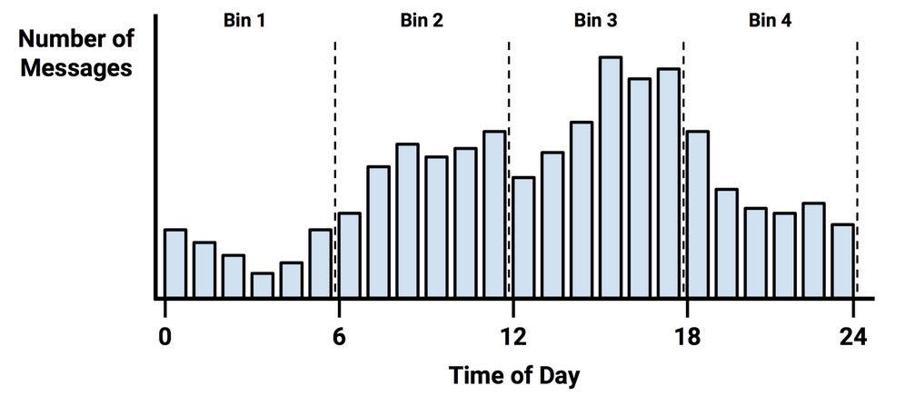
Figure 4.7: A histogram visualizing the distribution of the time emails were received
In the early hours of the morning, message frequency is low. Activity picks up during business hours and tapers off in the evening. This creates four natural bins of activity, as partitioned by the dashed lines. These indicate places where the numeric data could be divided into levels to create a new categorical feature, which could then be used with Naive Bayes.
The choice of four bins was based on the natural distribution of data and a hunch about how the proportion of spam might change throughout the day. We might expect that spammers operate in the late hours of the night, or they may operate during the day, when people are likely to check their email. That said, to capture these trends, we could have just as easily used three bins or twelve.
One thing to keep in mind is that discretizing a numeric feature always results in a reduction of information, as the feature's original granularity is reduced to a smaller number of categories. It is important to strike a balance. Too few bins can result in important trends being obscured. Too many bins can result in small counts in the Naive Bayes frequency table, which can increase the algorithm's sensitivity to noisy data.