Chapter 13. Introduction to classification

This chapter covers

• Why Mahout is a powerful choice for classification
• Key classification concepts and terminology
• The workflow of a typical classification project
• A step-by-step classification example

Life often presents us with questions that aren’t open-ended but instead ask us to choose from a limited number of options. This relatively simple idea forms the basis for classification—both that done by humans and that done by machines. Classification relies on the categorization of potential answers, and machine-based classification is the automation of such simplified decisions.

This chapter identifies those cases where Mahout is a good approach for classification and explains why it offers an advantage over other approaches. As an introduction to classification, this chapter also explains what classification is, and provides a foundation to understanding the basic terminology and concepts. In addition, we present a practical overview of how classification works, covering three stages in the workflow for typical classification projects: training the model, evaluating and tuning the model, and using the model in production. Following this introduction, we look at a simple classification project and show you, in a simple step-by-step way, how to put these basic ideas into practice.

13.1. Why use Mahout for classification?

Mahout can be used on a wide range of classification projects, but the advantage of Mahout over other approaches becomes striking as the number of training examples gets extremely large. What large means can vary enormously. Up to about 100,000 examples, other classification systems can be efficient and accurate. But generally, as the input exceeds 1 to 10 million training examples, something scalable like Mahout is needed. Table 13.1 shows the situations in which Mahout is most appropriate.

Table 13.1. Mahout is most useful with extremely large or rapidly growing data sets where other solutions are least feasible.

System size in number of examples	Choice of classification approach
< 100,000	Traditional, non-Mahout approaches should work very well. Mahout may even be slower for training.
100,000 to 1 million	Mahout begins to be a good choice. The flexible API may make Mahout a preferred choice, even though there is no performance advantage.
1 million to 10 million	Mahout is an excellent choice in this range.
> 10 million	Mahout excels where others fail.

The reason Mahout has an advantage with larger data sets is that as input data increases, the time or memory requirements for training may not increase linearly in a non-scalable system. A system that slows by a factor of 2 with twice the data may be acceptable, but if 5 times as much data input results in the system taking 100 times as long to run, another solution must be found. This is the sort of situation in which Mahout shines.

In general, the classification algorithms in Mahout require resources that increase no faster than the number of training or test examples, and in most cases the computing resources required can be parallelized. This allows you to trade off the number of computers used against the time the problem takes to solve.

The conceptual graph in figure 13.1 illustrates the advantages of scalable algorithms such as those in Mahout for medium to very large scale classification projects. When the number of training examples is relatively small, traditional data mining approaches work as well or better than Mahout. But as the number of examples increase, Mahout’s scalable and parallel algorithm is better with regard to time. The increased time required by non-scalable algorithms is often due to the fact that they require unbounded amounts of memory as the number of training examples grows. Extremely large data sets are becoming increasingly widespread. With the advent of more electronically stored data, the expense of data acquisition can decrease enormously. Using increased data for training is desirable, because it typically improves accuracy. As a result, the number of large data sets that require scalable learning is increasing, and as it does, the scalable classifiers in Mahout are becoming more and more widely useful.

Figure 13.1. The advantages of using Mahout for medium and large classification systems. The jagged line shows the effect of recruiting new machines to increase performance. Each new machine decreases training time.

13.2. The fundamentals of classification systems

Before looking at the way Mahout-based classification is done, let’s delve a little deeper into the basics of what classification is, and how it differs from recommendation and clustering.

Let’s first consider familiar examples of human-based classification. Filling in medical histories, completing surveys about the quality of a business’s service, or checking off the correct box for your filing status on tax forms—these are all situations where you make choices from a limited group of preselected answers. Sometimes the number of categories for responses is very small, even as few as two in the case of yes/no questions. In these situations, the classification process reduces what are potentially large and complicated responses to fit into a small number of options.

Definition

Classification is a process of using specific information (input) to choose a single selection (output) from a short list of predetermined potential responses.

Compare what happens to a person at a wine tasting to a person going to the store to get wine for dinner. At the wine tasting, people will ask, “What do you think of that wine?” and a wide range of answers are likely to be heard: “peppery,” “overtones of fruit,” “a rich finish,” “sharp,” “the color of my aunt’s sofa,” and “nice label.” The question is nonspecific, and the answers (output) don’t form a single selection from a predetermined short list of possibilities. This situation isn’t classification, though it may have some similarities to classification.

Now consider the wine shopper at the grocery store. Some of the same wine characteristics discussed at the wine tasting might matter to the shopper (taste, color, and so on), but in order to efficiently make the decision (to buy or not buy) and get to dinner, the shopper most likely has a mental checklist of simple characteristics to look for (red, $10, good with pizza, a familiar label), and for each bottle makes the decision (buy or don’t buy). Some detail and nuance may be lost, but simplifying the question to one that has very few potential answers (buy, don’t buy) is a practical way to make many decisions manageable. In this case, it gets the person out of the store in time for dinner. This situation is a form of classification.

Machines can’t do all the types of thinking and decision-making that humans do. But when the situation is within specific boundaries, machines can emulate human decisions efficiently in order to carry out classification. This machine-based approach can work when there is a single, focused decision, the input to be considered consists of a specific set of characteristics, and the output is categorical, which is to say, a single selection from a short list.

Classification algorithms are at the heart of what is called predictive analytics. The goal of predictive analytics is to build automated systems that can make decisions to replicate human judgment. Classification algorithms are a fundamental tool for meeting that goal.

One example of predictive analytics is spam detection. A computer uses the details of user history and features of email messages to determine whether new messages are spam or are relatively welcome email. Another example is credit card fraud detection. A computer uses the recent history of an account and the details of the current transaction to determine whether the transaction is fraudulent.

How do automated systems do this? We’d prefer them to do it magically, but in lieu of that, we rely on having them learn by example.

Definition

Computer classification systems are a form of machine learning that use learning algorithms to provide a way for computers to make decisions based on experience and, in the process, emulate certain forms of human decision making.

Classification algorithms learn by example, but they aren’t a substitute for human judgment, largely because they require carefully prepared examples of correct decisions from which to learn, and they require inputs that are carefully prepared for use in these algorithms. Unlike some other uses of Mahout, machine-based classification is a form of supervised learning.

13.2.1. Differences between classification, recommendation, and clustering

Classification algorithms stand in contrast to the clustering algorithms described in previous chapters because clustering algorithms are able to decide on their own which distinctions appear to be important (in machine learning parlance, they’re unsupervised learning algorithms) whereas classification algorithms learn to mimic examples of correct decisions (they’re supervised learning algorithms). Classification algorithms are also different from recommendation algorithms because they’re intended to make a single decision with a very limited set of possible outcomes, whereas recommendation algorithms select and rank the best of many possible alternatives.

Warning

One way to think about what classification is is to remind yourself of what classification is not: If your system is unsupervised, it is not classification. If your questions are open-ended or the answers aren’t categorical, your system is not classification.

Somewhat surprisingly, classification can be used creatively and effectively as a tool in a recommendation process. Typically, using a classifier to build a recommendation system isn’t as efficient as a real recommendation system, but the classifier as recommender can use some kinds of information that a normal recommendation system would have a hard time using. Recommendations systems normally use a history of what users have done, ignoring user and item characteristics that can be useful input for a classification system. The case study in chapter 17 will describe how a classifier can be useful as a recommender.

We’ve begun to answer the question, “What is classification?” Next we’ll look at what classification is used for.

13.2.2. Applications of classification

The output of a classification system is the assignment of data to one of a small predetermined set of categories. The usefulness of classification is usually determined by how meaningful the prechosen categories are. By assigning data to categories, the system allows the computer or a user to act on the output.

Classification is often used for prediction or detection. In the case of credit card fraud, a classifier can be useful in predicting which transactions will later be determined to be fraudulent based on known examples of behavior for purchases and other credit card transactions. The yes/no decision of whether or not a particular transaction is fraudulent is made by assigning that transaction to one of two categories: yes, fraud, or no, not fraud.

Classification is also valuable in predicting customer attrition in industries such as insurance or telecommunication. One way to design a classification system for this application is to train on data from a previous year’s records of known cases of attrition or retention, which are the categories being targeted as answers. Known characteristics of customers included in the training data set are selected as the features that can best predict whether or not a customer will stay with the service. Once trained, the classification system can be used to predict the future behavior of other customers based on the known, specific characteristics, including current behavior.

Note

Keep in mind that the term prediction, as used to describe what classifiers do, doesn’t refer solely to the ability to foresee future events. It also refers to the estimation of a value that may exist but not be easily available at the time of the classification.

Prediction can be the task of correctly assigning a characteristic (a category) based on available data rather than by directly testing for the characteristic. Often the characteristic that’s targeted for classification is itself too expensive to be determined directly, and that’s why classification becomes useful as a predictor. By expensive, we mean too costly in money or time or too dangerous.

For example, you may not want to wait a year or more to see telltale symptoms of a progressive illness, such as diabetes. Instead, you might build a classification system for early indicators of the disease that will assign risk in the future without having to wait until irreversible damage has possibly occurred. By knowing that a patient is pre-diabetic or likely to develop diabetes, doctors can provide options for prevention or early treatment.

Tip

Classification is often a way of determining the value of an expensive variable by exploiting a combination of cheap variables.

In related situations, a classification system can reduce physical danger. It’s preferable to be able to correlate data obtained by noninvasive means, such as cognitive tests or PET scans, to determine the existence of Alzheimer’s disease than to perform direct testing through autopsy on the brain, especially while the patient is still alive.

So classification can be useful. But why use Mahout instead of some other software?

13.3. How classification works

There are two main phases involved in building a classification system: the creation of a model produced by a learning algorithm, and the use of that model to assign new data to categories. The selection of training data, output categories (the targets), the algorithm through which the system will learn, and the variables used as input are key choices in the first phase of building the classification system.

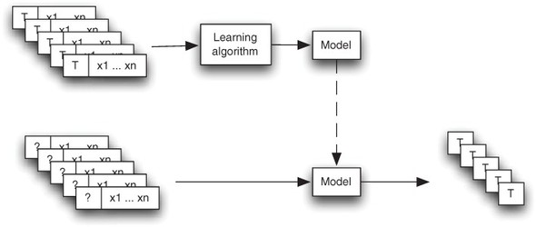
The basic steps in building a classification system are illustrated in figure 13.2. The figure shows two phases of the classification process: the upper path represents the training of the classification model; the lower path provides new examples to the model, which will assign categories (the target variables) as a way to emulate decisions. Input for the training algorithm consists of example data labeled with known target variables. The target variables are, of course, unknown to the model when using new examples during production. In evaluation, the value of the target variable is known, but it won’t be given to the model.

Figure 13.2. How a classification system works. Inside the dotted lasso is the heart of the classification system—a training algorithm that trains a model to emulate human decisions. A copy of the model is then used in evaluation or in production with new input examples to estimate the target variable.

For testing, which isn’t shown explicitly in figure 13.2, new examples that were withheld from the training data are presented to the model. The results chosen by the model are compared to known answers for the target variables in order to evaluate the model’s performance, a process described in depth in chapter 15.

The terminology used by different people to describe classification is highly variable. For consistency, we’ve limited the terms used for key ideas in the book. Many of these terms are listed in table 13.2. Note, in particular, the relationship between a record and a field: the record is the repository for values related to a training example or production example, and a field is where the value of a feature is stored for each example. The key ideas listed in this table are discussed in the subsections that follow.

Table 13.2. Terminology for the key ideas in classification

Key idea	Description
Model	A computer program that makes decisions; in classification, the output of the training algorithm is a model.
Training data	A subset of training examples labeled with the value of the target variable and used as input to the learning algorithm to produce the model.
Test data	A withheld portion of the training data with the value of the target variable hidden so that it can be used to evaluate the model.
Training	The learning process that uses training data to produce a model. That model can then compute estimates of the target variable given the predictor variables as inputs.
Training example	An entity with features that will be used as input for learning algorithm.
Feature	A known characteristic of a training or a new example; a feature is equivalent to a characteristic.
Variable	In this context, the value of a feature or a function of several features. This usage is somewhat different from the use of variable in a computer program.
Record	A container where an example is stored; such a record is composed of fields.
Field	Part of a record that contains the value of a feature (a variable).
Predictor variable	A feature selected for use as input to a classification model. Not all features need be used. Some features may be algorithmic combinations of other features.
Target variable	A feature that the classification model is attempting to estimate: the target variable is categorical, and its determination is the aim of the classification system.

In the following subsections, we look more closely at what a model is and how it’s trained, tested, and used in production. You’ll learn how to distinguish predictor variables from target variables, understand how to correctly make use of records, fields, and values, and see the four forms of values that variables can take. In addition, you’ll see that Mahout classification is an example of supervised learning.

13.3.1. Models

A classification algorithm learns from examples in a process known as training. The output of this training process is called a model. This model is a function that can then be applied to new examples in order to produce outputs that emulate the decisions that were made in the original examples. These emulated decisions are the end product of the classification system.

Note

The model produced by the training algorithm is itself effectively a computer program.

You saw in figure 13.2 how training examples, complete with desired output values, are given to the learning part of the classification system to create a model. This model, which itself can be viewed as a computer program that makes decisions, is then copied and given new examples as input. The intention is that the model will classify the new examples, emulating the training examples used as input.

13.3.2. Training versus test versus production

In practice, training examples are typically divided into two parts. One part, known as the training data, consists of 80–90 percent of the available data. The training data is used in training to produce the model. A second part, called the test data, is then given to the model without telling it the desired answers, although they’re known. This is done in order to compare the output of the model with the desired output.

Once the model performs as desired, it’s typically put into production and given additional examples to classify, for which the correct decision is unknown. Production results are usually not 100 percent accurate, but the quality of the output should stay consistent with what was achieved during the test runs unless the quality of the input data or external conditions changes.

It’s common to take samples of these production examples over time in order to make more training data, so that updated versions of the model can be produced. This sampling of production examples is important if external conditions might change, causing the quality of the decisions made by the model to degrade over time. In that case, a new model can be produced and the quality of the decisions can be improved or restored to original levels.

13.3.3. Predictor variables versus target variable

A variable is a value for a feature or characteristic of an example. The value can be derived by measurement or by computation. The ultimate goal of a classifier is to estimate a categorical answer to a specific question, and this answer is known as the target variable. In production, the target variable is the value being sought for each new example. In training, the target variable is known for historical data (training data) and is used to train the model.

In classification, the predictor variables are the clues given to the model so it can decide what target variable to assign to each example. Predictor variables used for classification are also known as input variables or predictors.

The characteristics of the examples to be classified can also be called features; the process of describing a particular characteristic in a way that can be used by a classification system is known as feature extraction. If a feature is chosen to be used as input for the model, the value of that feature would then be thought of as a predictor variable.

Recall the situation of the shopper buying wine for dinner. Attributes of the wine, such as “color,” “good with steak,” “good with fish,” “good with pizza,” and other attributes such as price are used by the shopper to make a decision to buy or not to buy. In the purchase decision, these features of the wine are analogous to predictor variables input to the model in machine classification. In this analogy, the decision has a binary target variable: buy or don’t buy. Only one of these choices will be selected for each bottle.

Note

Both the target and predictor variables are given to the learning algorithm during training. In contrast, during testing and in production, only the predictor variables are available to the model.

In preparing the classification system, the bulk of the historical examples used as training data will be labeled with the value of the target variable. During testing, the target variables for the test data will be cloaked. A comparison of the estimated target values produced by the model with the known values for each test example will reveal the accuracy of the classification model.

For classification, the field representing the target variable must have a categorical value. The value for predictor variables can be continuous, categorical, text-like, or word-like. You can see the differences between these types of values (continuous, categorical, text-like or word-like) in section 13.3.5. Often the target variable is a binary categorical variable, meaning it has only two possible values. Spam detection is an example of a classification system with a binary categorical variable: a message is spam or not spam. When there could be more than two possible values for the target variable, it’s called multi-class classification. An example of multi-class classification using data from 20 newsgroups is presented in chapter 14 (sections 14.4 and 14.6).

13.3.4. Records, fields, and values

The examples that comprise the input for classification algorithms are normally represented in the form of records. The A record can be thought of as a repository for the values of an example (whether a training example or a new example used in production). Records typically consist of a collection of named fields, each of which has a value.

The record for each training example will have fields to store values for the target variable and for one or more features chosen as predictor variables, as illustrated in figure 13.3. The field for the target variable in a production example is, of course, the unknown value that’s being sought by the classification algorithm. The output of the model in production is the value estimated for the target variable, denoted in the figure by T. There is one output for each input example.

Figure 13.3. Input and output of a classification model: target variables (T) and predictor variables (x1 ... xn). Notice that T is included with the input data during training but it’s absent from the input data in production (as indicated by?).

Although target values can only be categorical, several types of values can represent features used as predictor variables. We compare them next.

13.3.5. The four types of values for predictor variables

Predictor variables serve as the input for the learning algorithm, but which variables are useful depends in part on the type of values used to represent them. The distinction between different types of values for variables isn’t just an academic exercise. Your ability to correctly identify the types of values you have available will improve the success of your classification system.

There are four common types of values of predictor variables: continuous, categorical, word-like, and text-like, as described in table 13.3.

Table 13.3. Four common types of values used to represent features

Type of value	Description
Continuous	This is a floating-point value. This type of value might be a price, a weight, a time, or anything else that has a numerical magnitude and where this magnitude is the key property of the value.
Categorical	A categorical value can have one of a set of prespecified values. Typically the set of categorical values is relatively small and may be as small as two, although the set can be quite large. Boolean values are generally treated as categorical values. Another example might be a vendor ID.
Word-like	A word-like value is like a categorical value, but it has an open-ended set of possible values.
Text-like	A text-like value is a sequence of word-like values, all of the same kind. Text is the classic example of a text-like value, but a list of email addresses or URLs is also text-like.

Distinguishing between continuous and categorical values is often difficult. It’s a common mistake to treat numeric identifier codes as continuous values when they should really be considered categorical values. Consider, for instance, this list of values that represents the first three digits of ZIP codes: 757, 415, 215, 809, and 446. These values look numerical, and you might be tempted to consider them continuous, but they better fit the description of categorical because each one is from a set of prespecified values. Treating a value as continuous when it’s really categorical (or vice versa) can seriously impair the accuracy of a classifier.

Tip

Things that look like integers aren’t necessarily continuous. A key test is to imagine adding two values together or taking the log or square root of a value. If this doesn’t make any sense, then you probably have a categorical value rather than a continuous one. Another hint is that anything with an associated unit of measurement is usually a continuous variable.

A word-like value is an extension of categorical values to the point where there are many possible values. The distinction between these two types hinges on how many values a feature could have. Even if a feature could have many values, is there a finite group of prespecified values? In cases where you can’t say how many possible values there are, the variable likely is word-like. It’s often difficult to decide whether something should be treated as word-like or categorical. For instance, the combined make and model of a car might seem categorical, but if there is a good chance that a new car make or model could appear at any time, treating such a value as word-like might be a better choice.

In the occasional situation where categorical values have thousands or more possible values, they’re often better treated as word-like. If you already have many possible values, it’s likely that the set of values might not be as fixed as you might think. Occasionally, categorical values might have some ordering, but the classification algorithms in Mahout don’t currently pay attention to such ordering.

If you have a variable whose values can be viewed as collections of word-like values, you should consider it to be text-like, even if only a few examples might have more than one such value. Text-like values are often stored as strings and thus need a tokenizer that can convert the string representation as a sequence of word-like values.

Tip

A text-like variable can often be spotted by the fact that the components of the value can appear in almost any combination. For this reason, a variable that could have the values General Motors, Ford, or Chrysler isn’t text-like, even though General Motors appears to have two words in it. That’s because values like General Chrysler Ford don’t make sense.

Keep in mind the descriptions in table 13.3 as you examine table 13.4, which shows examples from different data sources. The first value, an email address, is a single entity from an open-ended set and thus is word-like. The values for spam words or non-spam words comprise a list of words (or possible words) and are considered text-like.

Table 13.4. Sample data that illustrates all four value types. These examples are typical of features of email data.

Name	Type	Value
from-address	Word-like	George <[email protected]>
in-address-book?	Categorical (TRUE, FALSE)	TRUE
non-spam-words	Text-like	Ted, Mahout, User, lunch
spam-words	Text-like	available
unknown-words	Continuous	0
message-length	Continuous	31

Note

Details of which types of predictor values are used by a particular algorithm are covered in chapter 14, section 14.5.

One of the distinctions between classification and other Mahout capabilities, such as clustering or recommendation, is based on whether learning is supervised or unsupervised. The next section explains this terminology.

13.3.6. Supervised versus unsupervised learning

Classification algorithms are related to, but still quite different from, clustering algorithms such as the k-means algorithm described in previous chapters. Classification algorithms are a form of supervised learning, as opposed to unsupervised learning, which happens with clustering algorithms. A supervised learning algorithm is one that’s given examples that contain the desired value of a target variable. Unsupervised algorithms aren’t given the desired answer, but instead must find something plausible on their own.

Supervised and unsupervised learning algorithms can often be usefully combined. A clustering algorithm can be used to create features that can then be used by a learning algorithm, or the output of several classifiers can be used as features by a clustering algorithm. Moreover, clustering systems often build a model that can be used to categorize new data. This clustering system model works much like the model produced by a classification system. The difference lies in what data was used to produce the model. For classification, the training data includes the target variables; for clustering, the training data doesn’t include target variables.

You now have a fundamental idea of what classification is, and you know about the advantages of using Mahout for classifying very large data sets. It’s time to put these ideas into practice.

13.4. Work flow in a typical classification project

Regardless of the differences between particular projects, there’s a pretty standard set of steps that need to be followed to build and run a classification system. In this section, we provide an overview of the typical workflow in classification projects: training the model, evaluating and adjusting the model to an acceptable level, and running the system in production. We look at an example using synthetic data to illustrate some of the steps in the workflow. We then look at a more complete example of this type in section 13.5 to complete a classification project using Mahout.

As a prerequisite to any project, you need to identify the information you’re seeking (the target variable) as a feature that can be stored in appropriate form in a record and that meets the overall goal, such as identifying a fraudulent financial transaction. Sometimes you’ll have to adjust what you choose as a target variable for pragmatic reasons, such as the cost of training, privacy issues, and so on. You also need to know what data is available for training and what new data will be available for running the system in order to design a useful classifier.

Note

Commonly, most of the effort required to build a classifier is spent inventing and extracting useful features. It’s also common to massively underestimate just how much work this step will involve.

The general steps in developing a classification project are listed in table 13.5. In each stage of the process, the accuracy of the system and the usefulness of the output largely reflect the original selection of features to be used as predictors and the categories chosen for the target variable. There isn’t a single, correct selection for each of these choices: a variety of approaches and adjustments are possible and experimenting with several is usually required to build an efficient and robust system.

Table 13.5. Workflow in a typical classification project

Stage	Step
Training the model	Define target variable. Collect historical data. Define predictor variables. Select a learning algorithm. Use the learning algorithm to train the model.
Evaluating the model	Run test data. Adjust the input (use different predictor variables, different algorithms, or both).
Using the model in production	Input new examples to estimate unknown target values. Retrain the model as needed.

Each step in the process of training and evaluating the model requires a balance between selecting features for variables that are practical and affordable in cost and time, and getting an acceptable level of accuracy in the values estimated by the model.

In the following sections, we discuss what happens during the three stages of classification.

13.4.1. Workflow for stage 1: training the classification model

In the first stage of a classification project, you need to have a target variable in mind, and this will help you select both appropriate historical data for the training process and a useful learning algorithm. These decisions go hand in hand.

No. 12

In the following discussion, we examine a few specific ways in which your choice of features will influence which Mahout learning algorithms will work in your classifier.

Define Categories for the Target Variable

Defining your target variable involves defining the categories for the target variable. The target variable can’t have an open-ended set of possible values. Your choice of categories, in turn, affects your choices for possible learning algorithms, because some algorithms are limited to binary target variables. Having fewer categories for the target variable is definitely preferable, and if you can pare the categories down to just two values, you’ll have a few more learning algorithms available to you.

If the target variable resists your efforts to reduce it to a simple form, you may need to build several classification systems, each deriving some aspect of your desired target variable. In your final system, you could then combine the outputs of these classification systems to produce the fully nuanced decision or prediction that you need.

Collect Historical Data

The source of historical data you choose will be directed in part by the need to collect historical data with known values for the target variable. For some problems, there will be difficulties in determining exactly what the value of the target variable should be.

The old saying about garbage in leading to garbage out is particularly apt here, and great care should be taken to make sure that the value of the target variable is accurate for the historical data. Many models have been built that faithfully replicate a flawed target variable or data collection process, and you don’t want to build another one.

Define Predictor Variables

After you have selected a useful target variable and have defined the set of values it can take on, you need to define your predictor variables. These variables are the concrete encoding of the features extracted from the training and test examples.

Once again, you’ll need to examine the source of your examples to make certain that they have useful features with values that can be stored in the appropriate format for their fields in the records. As you saw in figure 13.3, the predictor variables appear in records for the training and test data and for the production data.

Warning

A common mistake in selecting and defining predictor variables is to include what is known as a target leak in the predictor variables.

An important consideration in defining the predictor variables is to avoid setting up a target leak. A target leak, as the name implies, is a bug that involves unintentionally providing data about the target variable in the selection of the predictor variables. This bug isn’t to be confused with intentionally including the target variable in the record of a training example.

Target leaks can seriously affect the accuracy of the classification system. This problem can be relatively obvious when you tell the classifier that the target variable is a predictor, an error that seems obvious but that happens distressingly often.

Target leaks can be subtler as well. Suppose in building a spam detector, you keep the spam and non-spam examples in separate files and then label the examples sequentially within each file. Examples in the same file would have consecutive sequence numbers within a limited range and would have identical spam and non-spam statuses. With this type of target leak, many classification algorithms will quickly figure out the sequence number ranges that correspond to spam and to non-spam, and will settle on that one feature because it appears (in the training data) to be completely reliable. There lies the problem. When you give new data to a model that’s based almost entirely on sequence numbers, the best that the model could do is throw up its hands, because the sequence numbers in the new examples would be outside the previously seen ranges. More likely, the model would attribute new examples to whichever range had the highest sequence numbers.

Target leaks can be quite insidious and difficult to find. The best advice is to be suspicious of models that produce results that seem too good to be true.

Example 1: Using Position as a Predictor Variable

Let’s look at a simple example using synthetic data that illustrates how you can select predictor variables that will let a Mahout model accurately predict the desired target variable. The data displayed in figure 13.4 is a collection of historical data. Suppose you’re in search of filled shapes—color-fill is your target variable. What features will best serve as predictor variables for this problem?

Figure 13.4. Using position to classify color-fill: the target variable in this historical data is color-fill, and the features to be considered as predictor variables include shape and position. Position looks more promising as a predictor—the horizontal (x) coordinate may be sufficient. Shape doesn’t seem to matter.

For a classification problem, you must select categories for your target variable, which in this case is color-fill. Color-fill is clearly categorical with two possible values that you could label filled and unfilled. Or you could set up the target variable as a question with yes and no responses: “Is the item filled?”

Don’t take anything for granted: inspect the historical data to make certain it includes the target variable. Here it’s obvious that it does (good!), but in real world situations, it isn’t always obvious.

Now you must select the features for use as predictor variables. What features can you describe appropriately? Color-fill is out (it’s the target variable) but you can use position or shape as variables. You could describe position by the x and y coordinates. From a table of the data, you can create a record for each example that includes fields for the target variable and for the predictor variables you’re considering. A record for two of the training examples is shown in figure 13.5. (The complete data for this sample can be found in the examples module of the Mahout source code.)

Figure 13.5. Two records for training data. The records for data shown in figure 13.4 have fields that store the values of the target variable and fields for the values of the predictor variables. In this case, values relating to position (x, y coordinates) and shape have been included for each of the two examples.

If you once again examine the historical data depicted in figure 13.4, you’ll likely see that although the training data has both position and shape information, the x coordinate suffices to make the differentiation between filled and unfilled symbols. Shape has no utility in trying to determine whether a shape should be labeled as filled or not, nor does the y coordinate.

Tip

Not all features are useful for every classification problem. The specific situation and question you’re asking will determine which features make effective predictor variables. Learning about your data is crucial for success.

As you design your classification system, you’ll select those features that your experience suggests are most likely to be effective, and the accuracy of your model will tell you if you have chosen wisely. It isn’t necessary to exclude all features that aren’t useful in differentiation, but the fewer redundant or useless features you include, the more likely it is that your classifier will produce accurate results. For example, in the data shown in figure 13.4, you would do best to use only the x coordinate field for your final model and ignore the y coordinate and shape.

Example 2: Different Predictor Variables are Needed with Different Data

Just because a new collection of data exhibits the same features as a previous collection doesn’t mean you should use the same features as before for your predictor variables. This idea is illustrated in figure 13.6. Here you can see another collection of historical data that has the same features as the previous group. But in this situation, neither the x nor y coordinates seem helpful in predicting whether a symbol is filled or unfilled. Position is no longer useful, but shape is now a useful feature.

Figure 13.6. Using shape to classify color-fill: this data displays the same features (shape and position) as figure 13.4, but different predictor variables are needed to predict the target variable (color-fill). Here, position isn’t readily helpful, but shape is useful.

In this example, the feature chosen for a predictor variable (shape) has three values (round, triangle, square). Had it been necessary, you could also have used orientation to further differentiate shape (square versus diamond; upward-pointing triangle versus downward-pointing triangle).

Select a Learning Algorithm to Train the Model

In any project, you must select which algorithm to use, taking into consideration parameters such as the amount of training data, the characteristics of the predictor variables, and the number of categories in the target variable. Mahout classification algorithms include naive Bayes, complementary naive Bayes, stochastic gradient descent (SGD), and random forests. The use and behavior of naive Bayes, complementary naive Bayes, and SGD are described in detail in chapter 14 (section 14.5).

Even in these simplistic examples, different algorithms have different advantages. In example 1, the training algorithm should make use of the x coordinate position to determine color-fill. In example 2, shape is more useful. The x position of a point is, however, a continuous variable, and some algorithms can make good use of continuous variables. In Mahout, SGD and random forests do this. Other algorithms can’t use continuous variables, such as naive Bayes and complementary naive Bayes.

The improved speed of a parallel algorithm is obvious when you have an extremely large data set. Why, then, would you ever use the nonparallel (sequential) algorithm for classification? The answer is simply that there is a trade-off. The parallel algorithm does have considerable overhead, meaning that it takes a while to “find the car keys and get down the driveway” before it even begins processing any examples. Where you can afford the time, as with a medium-sized data set, the sequential algorithm may not only be sufficient but preferred. This trade-off is illustrated in figure 13.7, where the runtimes for hypothetical sequential and parallel scalable algorithms are compared.

Figure 13.7. Comparing two Mahout classifier algorithms. In both cases, the algorithms are scalable, as depicted in this conceptual graph.

Over the lower range of project sizes, the sequential algorithm provides a time advantage. In the midrange of size, both perform equally well. As the number of training examples becomes very large, the parallel algorithm outperforms the sequential one.

As explained for figure 13.1, the jagged shape of the parallel algorithm shows the times at which declining performance is revived by the addition of new machines.

Use Learning Algorithm to Train the Model

After an appropriate set of target variables and predictor variables have been identified and encoded, and a learning algorithm has been chosen, the next step in training is to run the training algorithm to produce a model (these steps were depicted in figure 13.3). This model will capture the essence of what the learning algorithm is able to discern about the relationship between the predictor variables and the target variable.

For example 1, the model would be something like the following pseudo-code:

if (x > 0.5) return FILLED;
else return UNFILLED;

Of course, a real model produced by a learning algorithm isn’t implemented this way, but this illustrates how simple a rule can be and still work in this example.

13.4.2. Workflow for stage 2: evaluating the classification model

An essential step before using the classification system in production is to find out how well it’s likely to work. To do this, you must evaluate the accuracy of the model and make large or small adjustments as needed before you begin classification.

Evaluating a trained model is rarely a simple process. Chapter 16 provides a detailed explanation of how to go about evaluating and fine-tuning a model in preparation for running the system in production. In the step-by-step example in section 13.5, you’ll see the beginnings of how evaluation works.

13.4.3. Workflow for stage 3: using the model in production

Once the model’s output has reached an acceptable level of accuracy, classification of new data can begin. The performance of the classification system in production will depend on several factors, one of the most important being the quality of the input data. If the new data to be analyzed has inaccuracies in the values of predictor variables, or if the new data isn’t an appropriate match to the training data, or if external conditions change over time, the quality of the classification model’s output will degrade. In order to guard against this problem, periodic retesting of the model is useful, and retraining may be necessary.

To do retesting, you need to gather new examples and verify or generate the value of the target variable. Then you can run these new examples as test data, just as in the second stage, and compare these results with the results of the original withheld data used in testing. If these new results are substantially worse, then something has changed and you need to consider retraining the model.

One common reason retraining becomes necessary is that the incorporation of the model into your system may change the system substantially. Imagine, for example, what happens if a large bank deploys a very effective fraud-detection system. Within a few months or years, the fraudsters will adapt and start using different techniques that the original model can’t detect as well. Even before these new fraud methods become a significant loss, it’s very important that the bank’s modelers detect the loss in accuracy and respond with updated models.

If the performance of a classification system has diminished, it’s probably not necessary to discard the approach. Retraining using new and more apropos training data may be sufficient to update the model. In addition, some adjustments to the training algorithm can be useful. Ongoing evaluation is a part of retraining, as described in more detail in the discussion of model updates in chapter 16 (section 16.4.1).

13.5. Step-by-step simple classification example

You’ve now learned the basics of what classification is, and how the workflow progresses in a typical project. You’ve seen the importance of carefully selecting which features to use as predictor variables based on the question you’re asking and which target variables you’re estimating.

Although Mahout is intended for extremely large data sets, it’s helpful to start with a simple example as you familiarize yourself with Mahout. In this section, you’ll have a chance to put Mahout into action as a classifier for a small practice data set. We describe the data involved, how to train a model, and how to tune the classifier a bit for better accuracy.

13.5.1. The data and the challenge

In this section, you’ll train a classification model to assign color-fill to a collection of synthetic data similar to those in the previous sections. In the training data, the target variable once again will be color-fill, having two categories: filled and not filled. In this data, position is the key to predicting color-fill, and you’ll use a Mahout classification algorithm called stochastic gradient descent (SGD) to train the model.

The historical data for this do-it-yourself practice project is depicted in figure 13.8 and is included as part of the Mahout distribution. To help you get started with classification, Mahout has several such data sets built into the JAR file that contains the example programs. We refer to this data set as the donut data.

Figure 13.8. Example 3 data for a simple classification project: the donut data. What features are useful for finding filled points?

For this simple classification project, the target variable is color-fill, and your goal is to build a system capable of finding filled points.

13.5.2. Training a model to find color-fill: preliminary thinking

As you consider how to train a model for your project, think about what will work as predictor variables. In the example discussed in section 13.3.1 and depicted in figure 13.4, position rather than shape was key. A cursory inspection of figure 13.8 tells you that for this simple collection of data, position is once again key. But you may suspect that neither x nor y coordinates, nor a combination of the two, are likely to be sufficient to predict the location of filled points for this data set.

For a feature such as position, there is more than one way to consider it as a variable. Perhaps position defined as distance to a particular fixed point such as A, B, or C would be useful, as shown in figure 13.9.

Figure 13.9. If position is the feature used as the predictor variable for this donut data set, you must decide how best to designate position to achieve your particular goal—to identify filled points. The distance to C looks the most useful.

Although x and y coordinates are sufficient to specify any particular point, they aren’t useful features to predict whether a point is filled. Adding the distances to points A, B, and C restates position in a way that makes it easier to build an accurate classifier for this data. Distance to C is promising, but you may choose to include additional predictor variables in your system. The details for doing this are described in the following sections.

13.5.3. Choosing a learning algorithm to train the model

Mahout provides a number of classification algorithms, but many are designed to handle very large data sets and as a result can be a bit cumbersome to use, at least to start. Some, on the other hand, are easy to get started with because, though still scalable, they have low overhead on small data sets.

One such low overhead method is the stochastic gradient descent (SGD) algorithm for logistic regression. This algorithm is a sequential (nonparallel) algorithm, but it’s fast, as was shown in the conceptual graph in figure 13.9. Most importantly for working with large data, the SGD algorithm uses a constant amount of memory regardless of the size of the input.

Start Running Mahout

First, download and unpack Mahout from mahout.apache.org. Assuming that you put the unpacked directory name in the MAHOUT_HOME environment variable, you can list the commands available with the command-line tool in Mahout:

$ $MAHOUT_HOME/bin/mahout
An example program must be given as the first argument.
Valid program names are:
  canopy: : Canopy clustering
  cat : Print a file or resource as the logistic regression models would see
     it
...
  runlogistic : Run a logistic regression model against CSV data
  ...
 trainlogistic : Train a logistic regression using stochastic gradient
     descent
 ...

The commands that we’ll be most interested in here are the cat, trainlogistic, and runlogistic commands.

Check Mahout’s Built-in Data

To help you get started with classification, Mahout includes several data sets as resources in the JAR file that contains the example programs (see the examples/src/ main/resources/ directory). When you specify an input to the SGD algorithm, if the input you give doesn’t specify an existing file, the training or test algorithm will read the resource of that name instead, if a resource of that name exists.

To list the contents of any of these resources, use the cat command. For instance, this command will dump the contents of the donut data set illustrated in figure 13.8:

$ bin/mahout cat donut.csv
"x","y","shape","color","k","k0","xx","xy","yy","a","b","c","bias"
0.923307513352484,0.0135197141207755,21,2,4,8,0.852496764213146,...,1
0.711011884035543,0.909141522599384,22,2,3,9,0.505537899239772,...,1
...
0.67132937326096,0.571220482233912,23,1,5,2,0.450683127402953,...,1
0.548616112209857,0.405350996181369,24,1,5,3,0.300979638576258,...,1
0.677980388281867,0.993355110753328,25,2,3,9,0.459657406894831,...,1
$

Note that most of the contents aren’t shown, as indicated by the ellipsis (...). This file consists of a first line that specifies the names of the fields in the data, followed by more lines that contain the data itself. As you can see, the original predictor variables that we talked about are included: x, y, shape, and color. The values of x and y are numerical values in the range [0, 1] whereas shape is an integer in the range [21 ... 25]. The color is an integer that’s always 1 or 2. Because subtracting a triangle from a square makes no sense, we should consider the shape variable to be categorical. Likewise, the color values should be considered numerical codes for a categorical variable with two values.

In addition to x, y, shape, and color, there are additional variables present in this data to allow you to experiment with different classification schemes. These variables are described in table 13.6.

Table 13.6. Fields used in the donut.csv data file

Variable	Description	Possible values
x	The x coordinate of a point	Numerical from 0 to 1
y	The y coordinate of a point	Numerical from 0 to 1
shape	The shape of a point	Shape code from 21 to 25
color	Whether the point is filled or not	1=empty, 2=filled
k	The k-means cluster ID derived using only x and y	Integer cluster code from 1 to 10
k0	The k-means cluster ID derived using x, y, and color	Integer cluster code from 1 to 10
xx	The square of the x coordinate	Numerical from 0 to 1
xy	The product of the x and y coordinates	Numerical from 0 to 1
yy	The square of the y coordinate	Numerical from 0 to 1
a	The distance from the point (0,0)	Numerical from 0 to
b	The distance from the point (1,0)	Numerical from 0 to
c	The distance from the point (0.5,0.5)	Numerical from 0 to
bias	A constant	1

Build a Model Using Mahout

You can build a model to determine the color field from the x and y features with the following command:

$ bin/mahout trainlogistic --input donut.csv 
       --output ./model 
       --target color --categories 2 
       --predictors x y  --types numeric 
       --features 20 --passes 100 --rate 50
...
color ~ -0.157*Intercept Term + -0.678*x + -0.416*y
       Intercept Term -0.15655
                    x -0.67841
                    y -0.41587
...

This command specifies that the input comes from the resource named donut.csv, that the resulting model is stored in the file ./model, that the target variable is in the field named color and that it has two possible values. The command also specifies that the algorithm should use variables x and y as predictors, both with numerical types. The remaining options specify internal parameters for the learning algorithm.

Note

The actual output you see will probably only agree to one significant figure because the logistic regression training algorithm used is somewhat randomized.

A list of all of the command-line options for the trainlogistic program is shown in table 13.7.

Table 13.7. Command-line options for the trainlogistic program

Option	What it does
--quiet	Produces less status and progress output.
--input <file-or-resource>	Uses the specified file or resource as input.
--output <file-for-model>	Puts the model into the specified file.
--target <variable>	Uses the specified variable as the target.
--categories <n>	Specifies how many categories the target variable has.
--predictors <v1> ... <vn>	Specifies the names of the predictor variables.
--types <t1> ... <tm>	Gives a list of the types of the predictor variables. Each type should be one of numeric, word, or text. Types can be abbreviated to their first letter. If too few types are given, the last one is used again as necessary. Use word for categorical variables.
--passes	Specifies the number of times the input data should be re-examined during training. Small input files may need to be examined dozens of times. Very large input files probably don’t even need to be completely examined.
--lambda	Controls how much the algorithm tries to eliminate variables from the final model. A value of 0 indicates no effort is made. Typical values are on the order of 0.00001 or less.
--rate	Sets the initial learning rate. This can be large if you have lots of data or use lots of passes because it’s decreased progressively as data is examined.
--noBias	Eliminates the intercept term (a built-in constant predictor variable) from the model. Occasionally this is a good idea, but generally it isn’t since the SGD learning algorithm can usually eliminate the intercept term if warranted.
--features	Sets the size of the internal feature vector to use in building the model. A larger value here can be helpful, especially with text-like input data.

13.5.4. Improving performance of the color-fill classifier

Now that you have trained your first classification model, you need to determine how well it’s performing the task of estimating color-fill condition. This evaluation stage isn’t just a way to assign a grade for your project. It’s your means of assessing and improving your classifier for excellent performance.

Evaluate the Model

Remember that this problem has the filled points completely surrounded by unfilled points, which makes it impossible for a simple model, such as is produced by the SGD algorithm using only x and y coordinates, to classify points accurately. Indeed, the linear equation underlying this model can only produce a negative value, which, in the context of logistic regression, is guaranteed to never produce a score greater than 0.5. As we shall see, this first model isn’t very useful.

After the model is trained, you can run the model on the training data again to evaluate how it does (even though we know it won’t do well).

$  bin/mahout runlogistic --input donut.csv --model ./model 
        --auc --confusion
AUC = 0.57
confusion: [[27.0, 13.0], [0.0, 0.0]]
...

The output here contains two values of particular interest. First, the AUC value (an acronym for area under the curve—a widely used measure of model quality) has a value of 0.57. AUC can range from 0 for a perfectly perverse model that’s always exactly wrong to 0.5 for a model that’s no better than random to 1.0 for a model that’s perfect. The value here of 0.57 indicates a model that’s hardly better than random.

To understand why this model performs so poorly, you can look to a confusion matrix for a clue. A confusion matrix is a table that compares actual results with desired results. All examples at the default score threshold of 0.5 are classified as being unfilled. This allows the classifier to be correct two-thirds of the time (27 out of 40 times), but it only manages to be correct marking everything as unfilled. This model gets the right answer much of the time, but only in the way that a stopped clock is right twice a day.

Note

Along with other measurement tools, the confusion matrix is described in more detail in chapter 15.

The options accepted by the runlogistic command are summarized in table 13.8.

Table 13.8. Command-line options for the runlogistic program

Option	What it does
--quiet	Produces less status and progress output.
--auc	Prints AUC score for model versus input data after reading data.
--scores	Prints target variable value and scores for each input example.
--confusion	Prints confusion matrix for a particular threshold (see --threshold).
--input <input>	Reads data records from specified file or resource.
--model <model>	Reads model from specified file.

Build a More Interesting Model

You can get more interesting results if you use additional variables for training. For instance, this command allows the model to use x and y as well as a, b, and c to build the model:

$ bin/mahout trainlogistic --input donut.csv --output model 
         --target color --categories 2 
         --predictors x y a b c  --types numeric 
         --features 20 --passes 100 --rate 50
...
color ~ 7.07*Intercept Term + 0.58*x + 2.32*y + 0.58*a + -1.37*b + -25.06*c
       Intercept Term 7.06759
                    a 0.58123
                    b -1.36893
                    c -25.05945
                    x 0.58123
                    y 2.31879
...

Notice how this model applies a large weight to the c variable, as well as a large intercept term. If you ignore the other variables (which isn’t entirely appropriate to do, but the intercept and c are definitely dominant here), the output of the linear part of this model will reach a maximum value of 11.5 where c = 0, and it will drop rapidly into negative territory once c > 0.3. This makes a lot of sense geometrically, based on what we know about the problem. This consideration alone is a strong indication that this isn’t a stopped-clock model like the one that depended on x and y alone.

Test Again

If you run this revised model on the training data, you’ll get a very different result than with the previous model:

$  bin/mahout runlogistic --input donut.csv --model model 
         --auc --confusion
AUC = 1.00
confusion: [[27.0, 0.0], [0.0, 13.0]]
entropy: [[-0.1, -1.5], [-4.0, -0.2]]

Now you have a perfect value of 1 for AUC, and you can see from the confusion matrix that the model was able to classify all of the training examples perfectly.

Test Using New Data

You can run this same model on additional data in the donut-test.csv resource. Because this new data was not used to train the model, there are a few surprises in store for the model.

$  bin/mahout runlogistic --input donut-test.csv --model model 
          --auc --confusion
AUC = 0.97
confusion: [[24.0, 2.0], [3.0, 11.0]]
entropy: [[-0.2, -2.8], [-4.1, -0.1]]

On this withheld data, you can see that the AUC has dropped to 0.97, which is still quite good. The confusion matrix shows that of the 40 new samples, there are 5 incorrectly classified examples, 2 unfilled points that were marked as filled by the model (false positives), and 3 filled points that were marked by the model as unfilled (false negatives). Clearly the use of the additional variables, notably the inclusion of c, has helped the model substantially, but there are still a few issues. Figure 13.10 shows what happened.

Figure 13.10. Trying the classifier on new data. The original data is shown in a lighter shade, and the new data is shown filled or not. The enlarged symbols are the ones that the model got wrong. The diamond outline shows the region that we actually used to generate the donut data.

Notice the large, filled circle near the bottom of the diamond in figure 13.10. This circle is close to training dots that weren’t filled, but it’s not near any filled training dots. Because the learning algorithm wasn’t allowed to know that the correct region had this odd shape, it was nearly impossible for the model to get the right answer.

Try Other Models

You can do additional experiments by selecting other sets of variables. For instance, here is what happens when you include x, y, a, and b, but exclude c from the set of predictor variables:

$ bin/mahout trainlogistic --input donut.csv --output model 
           --target color --categories 2 
           --predictors x y a b  --types n --features 20 
           --passes 100 --rate 50
...
color ~ 4.634*Intercept Term + -2.834*x + 5.558*y + -2.834*a + -6.000*b
       Intercept Term 4.63396
                    a -2.83439
                    b -5.99971
                    x -2.83439
                    y 5.55773
  ...
$  bin/mahout runlogistic --input donut-test.csv --model model 
             --auc --confusion
AUC = 0.91
confusion: [[27.0, 13.0], [0.0, 0.0]]
   entropy: [[-0.3, -0.4], [-1.5, -0.7]]
$

This time, the model does only slightly worse on the withheld data, even though it didn’t have access to its favorite variable. This indicates that the information carried by c is also available in x, y, a, and b.

You can try lots of experiments on the parameters of the learning model, as well. These experiments are the beginning of the evaluation process described in chapter 15.

13.6. Summary

By developing the example in the previous section, you’ve put to use what you learned throughout this chapter about the first two stages of classification: how to train a model and how to evaluate it and adjust performance. If this were a real system, your model would now be ready for the third stage in classification: deploying it into production in a real-world setting. The basic terminology of classification will now be familiar to you, and you should have a solid understanding of what classification is and how it works.

Remember that an important key to building a successful classifier is to carefully pose your question in specific and simple terms so that it can be answered by a limited list of predetermined categories, the target variables. Be aware that not all features of the input data are equally helpful; you must select the features to be used as predictor variables carefully, and you may need to try many combinations to find which ones are useful for your classifier to perform well. And remember, pragmatism is important.

With these ideas in mind, think back to the example of wine tasting. The goal of your machine-based classifier should be to help you get to dinner on time, not to help you make subtle aesthetic judgments about the finer things in life.

As you continue through chapters 14–17, you’ll see how Mahout provides a powerful tool to meet the requirements of extremely large classification systems, particularly those with data sets above 1 million examples. Chapter 14 focuses on how to extract features for input to the learning algorithm as a first step in finding out how to evaluate and tune a trained classifier before deploying it to production.