Introduction
The first two chapters of this book provided reasons to use system dynamics (SD) modeling in a company or organization and enough brief guidelines to understand, and perhaps experiment with, iThink models and modeling with their trial software.
This chapter provides some detailed guidance on how to start such a project if the reader is interested in doing so. The guidance in this chapter comes from a multitude of sources, unlike that in Chapter 2. I have drawn on Richmond, but also on an online course, a number of other resources that I will identify as we progress through the chapter, and of course, my own experience with modeling, both directly and indirectly.1
The intention is to give the user, perhaps a first-time modeler, a sufficient understanding of the process to get started. While this is always best undertaken with the knowledge and support of others in the organization, that adds the complexities of group dynamics and coordination and enlarges the scope of the job. It is entirely possible to begin a modeling project on one’s own, just to see what might be there with respect to a particular question. While done for academic reasons, Hall’s work was essentially a one-man show, and many in the consulting or support fields might find it useful to work by themselves, if not for the entire project then for a beginning period.2
Following a brief look into the application of SD modeling, I provide a number of general guidelines and requirements for doing it, followed by several suggestions for some specific techniques that I consider best practices. As we will see, there are a number of ways to approach modeling, whether as a one-man show or as a larger team effort, and each creates some unique challenges as well as unique opportunities.
Application of SD Modeling
In recent years, companies have been applying dynamic modeling as a management tool to a greater extent than ever before. Among Scandinavian companies, nearly 30 percent of firms were reported to regularly use simulation tools as aids to strategy formulation and decision making.3 This evidently is a growing category of business applications and, in the right hands, adds considerable economic value and competitive advantage to those firms.
Getting data on U.S. adoptions of SD modeling is more difficult for a number of reasons, perhaps the most important being that if SD modeling works, it is best kept a competitive secret. The Systems Dynamics Society maintains a collection of application cases, and its corporate case list has only 21 items out of total of 54, but 22 government organizations and 11 nongovernment organizations also report using it. Procter & Gamble, the global consumer goods company, uses simulation as one of four major types of “operations research” tools to support similar functions;4 Dow Chemical is reported to have used iThink to improve supply chains;5 but little else is heard from the business community, and I suspect this is a case of “Macy’s not telling Gimbels.”6
There are other potential reasons for not reporting usage as well: since many enterprise resource planning (ERP) systems encompass most functional areas of client businesses, they have some power to perform simulation or to support other systems that do it through decision support (even if more limited than true SD modeling). Thus, it is likely that businesses do not report using modeling because “everyone does it” and there is nothing particularly novel about it. I should acknowledge this as my interpretation of these systems and their use; I should also point out that ERP systems are not true SD modeling software. A major difference is that SD attempts to look at systems very parsimoniously, without trying to take into account all possible variables that might affect one; ERP, on the other hand, must account for all details, and is not intended to ask whether the current system structure is the right one. But many ERP programs do have some capability to ask “what if” questions.
We should not overlook the potential for SD modeling to reveal previously unseen organizational problems. One study suggests that despite the dramatic improvements in manufacturing (in terms of product yield, cycle time, and product defects), a total quality management program affected installed accounting systems and organizational processes so severely that excess capacity was created, leading to pressure for layoffs and attendant stresses, and the result was that support for the program was greatly diminished. SD modeling of this company strongly suggested that unexpected feedback loops in the firm created serious conflict between short-term and long-term performance goals; it is quite easy to envision how such news might be quashed.7
Whatever the reason, we know little beyond the advertising claims for the adoption of ERP modeling. As noted in Volume I, not all ERP applications succeed, and many are apparently undertaken on faith of their payoff.
Creating and Using SD Models
Map, Then Model
Successful dynamic modeling requires a thorough understanding of the major variables and the relationships between them in the workflow(s) being modeled. Workflow Mapping and Analysis (WFMA) provides the basic information for development of a dynamic model. A validated map, as described in Volume I, is usually the best place to start simply because it is a valid map. This establishes a baseline for both initial construction of the model and for testing it to determine if we have translated the workflow map into a model correctly.
The need for “translation” arises because the symbols and terminology used in dynamic models are different from those we use in WFMA, as we now know—dynamic models consist of “stocks,” “flows,” and “rates,” and the WFMA workflow map data we begin with must be converted into these variables in the SD model. Not surprisingly, the primary type of variable captured in a workflow map is termed a “flow” or “converter” in dynamic modeling; these flows will be linked to one or more stocks, or accumulations, of both input and output materials at the beginning and end of the workflow cycle, and the converters will modify the flows. What happens in the course of the workflow will consist of several possibilities that we must translate. One is that between the beginning and end of the workflow there may be one or more types of “work in process” that are intermediate transformations of information and material into something different, but not yet their final form. These may be defined as intermediate stocks and flows in cases where material passes through several steps or subprocesses in transformation.
A second type of translation is concerned with points in the workflow where material flows may diverge or be parsed into different categories. These will nearly always be associated with a decision point in a workflow (a decision diamond in the map), since these are the only places where materials can be redirected. An obvious example is in the area of quality control, where one might complete the assembly of some item and then come to a quality control point, where the question is “does this unit meet specifications?” If the answer is “no,” that unit is removed as defective. The translation of this process into a “rate” is to determine what percentage of assembled units fail this test, and then use this figure as the appropriate converter for lost production (or use the success rate if preferred). Most decision diamonds, however, are purely informational and will often be translated into converters.
It may be helpful to think in terms of all possible outcomes of a workflow and how these can be categorized. Figure 3.1 is a WFMA map of a fairly typical quality control process in manufacturing, in which items are sampled from a production run and returned if they are within specifications. Items not “on spec” may be repairable, and if so, they are repaired, reinspected, and returned to the flow of finished goods (assuming they meet specification on reinspection). Items not repairable are simply scrapped.
Figure 3.2 summarizes the outcomes of the workflow in Figure 3.1, in terms of normal or exception-handling outcomes, either of which can be a success or a failure. Regular production successes (which can be the output of successful innovation processes as well) are in the upper left cell of the figure. Successful exception-handling outcomes are directly beneath successful production in the lower left cell. In many cases, unsuccessful normal production may be an exception to be corrected, so it is possible that a successful exception-handling process may result in no loss to “regular” production, because those items return via the exception-handling process; it may also be possible that an exception that costs more to correct than the value it adds will simply be discarded.

Figure 3.1 A WFMA map of a manufacturing quality control process

Figure 3.2 Exhaustive categorization of process outcomes
Failures can occur in either case, and these are shown in the right column of Figure 3.2. Undetected flaws (which might have been subject to correction had they been caught) are an undesirable residual of the quality control process, and are sent into the environment (customers) to be detected there. Unsuccessful exception-handling processes result in “scrap” for the most part, regardless of what we call it.
Any of the outcomes in Figure 3.2 can be regarded as a “stock” in dynamic modeling terms, and the processes that create each of them a “flow,” where parts of some flows will probably overlap. (We will probably express stocks on the failure side of the figure as converters, serving as stock substitutes; this can also be done for the bottom-left stock, so that we would have only one true “stock” in the four cells.) If we have measures of the four outcomes, which is likely with the exception of undetected flaws, then much of the basic information needed to construct a dynamic model is in hand. If not, we have at least identified processes that should be sampled and measured to provide the data we need. Such samples may be useful for SD modeling or in static modeling as discussed in Volume I.
Figure 3.3 shows what the workflow map in Figure 3.1 looks like when translated into a dynamic model in iThink software. Raw materials are brought from their sources (represented as a “cloud” icon) through a flow, and become a “stock” of work in process, illustrated as a “ conveyor.” The production flow is sampled for inspection, shown by the solid “action” arrow from initial production to the inspection process (shown as a module, discussed in the “Next Steps” section).8 Inspection uses a set of data and procedures in their process (not shown in this version of the module) to determine whether sampled items are within specifications or not—those within spec are returned to the stock of finished goods, and those not acceptable or repairable are rejects, which are a loss of finished-goods salable inventory; the rate of rejects signifies a reduction in the available products for customers. Using the module to describe this process is consistent with iThink 10.0 and above. The inspection module can be expanded to show the rework-and-reinspect process in Figure 3.1. All of the possible outcomes in either Figure 3.1 or 3.2 can occur in the dynamic model shown in Figure 3.3, but the diagram in Figure 3.3 is quite unlike the WFMA maps we have seen in Volume I.
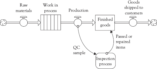
Figure 3.3 Basic iThink model of manufacturing quality control process shown in Figure 3.1
Some of the symbols used in Figure 3.3 are familiar WFMA symbols with similar meanings, but others are particular to iThink and bound by the unseen programming rules that are in turn driven by the diagram in Figure 3.3. Given the fact that these diagrams literally create a mathematical model of the process, these restrictions are necessary. These rules mean, as mentioned earlier, that considerably more effort will be needed to create dynamic models than to create static workflow maps because the rules of iThink are more restrictive than WFMA and the objective of the SD model is to simulate the overall process.
This general approach of translating WFMA maps into dynamic models can be scaled down to the subprocesses within larger streams of activity if desired, and can also be scaled up to apply to higher-level systems, given that we have sufficient data at each level for the model. A caveat in all cases is to beware of getting “down into the weeds,” and attempting to make the model a replication of the complete larger system.9 Any such up- or down-scaling, however, depends on the data about processes available to the modeler; translation from a valid static model to an SD model requires not only knowledge of the process but valid process data.
Simulation Data Requirements
As a static model, WFMA can produce data for analysis. Unlike static models, dynamic simulation requires prior definition of system states in terms of data and information which reflects the inputs the system acquires and outputs the system produces in order for the model to run. There are frequently many intermediate states of production and ancillary processes that may also need to be specified. To model any system, data, which can both inform the model on the properties of the inputs and can generate representative final and intermediate outputs, will be required.
We are already familiar with two types of data requirements, for stocks and flows. For many WFMA analyses, we will be measuring these as incoming and outgoing inventory levels (whether in the form of manufactured parts, incoming and outgoing patients or students, documents processed or awaiting processing, or whatever it is that we do). The most common data created by a workflow map has to do with completion of the workflow process, and that may go through a number of steps that may or may not be measured.
For dynamic simulation, a third type of data will be needed, and that is the rate of movement of many of these items. We are all familiar with many kinds of rates and use them in everyday discussion. In education, we are interested in both the percentage of students who excel as well as the percentage who fail; in hospitals we are concerned with the rate of patient infection, expressed as a percentage or (hopefully) as the number on a larger base, perhaps the number of infections per thousand admissions; we measure speed as distance over time, and in most of the world as kilometers per hour (kph) or miles per hour (mph) in the United States.
Rates are changes over some base value, usually expressed as a percentage or fraction, and they are used as converters in SD models in many ways. In Figure 2.9, for example, we see rates expressed as decay on the left, and adjustment time and a perception gap on the right. Rates can often be expressed as positive or negative values; “positive” and “negative” sometimes connote meanings other than mathematical, as noted in Chapter 2, and for that reason I recommend description of rates in the most neutral language possible.
Rates may be calculated from basic data measured on a workflow map. Many WFMA process-map outputs can be converted into rates by dividing them by the appropriate time unit; in other cases, data will need to be collected or modified to convert them to rates. In Figure 3.1 we could measure the number of items sampled, the number on spec, the number not on spec but repairable, and so on for most steps in the workflow. We can also measure total production over time for the entire process (units per minute or hour or day, as appropriate). We can measure the time required to complete an inspection, and the length of time an item spends in the repair–reinspect–return or discard subprocess. With a valid workflow map and measures taken from what is actually being done in the workflow, acquiring or creating meaningful rate information is usually greatly simplified, and confidence in the simulation models based on the data is enhanced.
This is not always the case, however. One of the frustrations that can afflict many modelers is that once a system workflow is mapped and understood, we may find there are neither metrics nor measurement processes that capture the data needed to model the system. In my Navy research, I was often astounded to find that information I assumed had been captured somewhere in the system had not been captured. For example, in the early days of examining the performance of the Versatile Avionics Shop Test (VAST) shops, I found that there had never been a requirement for benchmark “standard” times to be available for all of the avionics components serviced by the VAST tester. My interests in this information were several, not the least being able to get an idea of “how badly VAST was performing” against its intended capabilities, if it was the culprit in the maintenance workflow that so many believed it to be. Lacking that, I went looking for some average data on repair activity—I knew that the Navy collected the clock times for every AC that entered and left the repair process in the VAST shop when the item was serviced, and I thought surely someone had crunched the numbers to get some idea what the averages were. None ever had, so I thought certainly there must be some such information on the really difficult-to-repair ACs that so often seemed to jam up the system, but that was not the case, either. To complete my research on this part of the repair cycle, I had to take nearly a year to get the raw data from the Navy, hire a graduate assistant, and then extract what we needed from scratch.
This is not a phenomenon that applies only to the factory floor or the maintenance cycle. Recent interest in “evidence-based medicine,” in large part, is partly derived from belated recognition of the lack of output data possessed by the medical profession—in short, there are many drugs and medical and surgical procedures, which produce highly variable final results. Only now is the profession beginning to take steps to measure and evaluate these outcomes, with a major objective being to validate procedures that until now have largely been taken on faith.10
In my own experience, this can be one of the more frustrating aspects of SD modeling, and in some cases a cause for dynamic models to get a “bad rap.” Users will complain that an SD model does a very poor job of representing a system and generates outputs that are contrary to history and everyday experience. In the cases I have worked with, this has usually been attributable to poor understanding of the system in the first place, that is, that valid static models were not generated as a baseline for dynamic modeling, or in other instances, the modelers wanted to model the system that “should be,” only to learn that it produced many outputs that should not be. Translating these into SD models does not improve them.
Guidelines and Suggestions for SD Modeling
As I mentioned earlier, the beginning of a modeling project may be a group effort or a one-person undertaking. Personally, I prefer to work with a team of people who are interested in an organizational problem and are motivated to understand it before trying any “fixes.” But some problems or issues are of more personal interest, or may be a problem awaiting “discovery” before attracting attention, and so on; in any case, these may be more suited to initial individual attention. In either case, many of the same suggestions will apply, and if there are circumstances where I need to differentiate my suggestions for group or individual projects, I will note that. In presenting these guidelines, I have again drawn on a number of earlier writers in the field, but have also added some suggestions based on my own experience with modeling, and interaction with managers and others who have used it.
The first thing one has to do in developing an SD model is to learn patience. This advice is not commonly given by the various texts and writings on the subject, but is something I have learned is necessary to do modeling successfully; and, I must admit, this has been a hard lesson for me. As a typical American, I have a strong desire to get things done and move on to the next item on my list, and this is a trait that I have found in many of my trainees and students. But this is something that one must learn to temper and control; when engaging in SD modeling, the essential nature of the model is what matters most, not the myriad details that accompany it. It is the process of identifying what should be included in the model, and perhaps more importantly, what should not be—neither of these is likely to be obvious or readily teased out of the details. Thinking, comparison, questioning, and consulting with others are needed, and all these take time.
Most company and organizational modeling projects will be over issues that are often more complex than meets the eye. Many ideas about the “cause” and “effect” of different variables will have become entrenched, and in many cases, will be partially correct and partially incorrect, all at the same time. The best way to bound and define these problems is to have a conversation about what is perceived by different individuals. In my own case, I was struck by a parallel between my experience with the Naval Air Systems Command (NAVAIR) studies and Hall’s research into the demise of the Saturday Evening Post,11 discussed in Chapter 1— while there were only a few variables that the managers in either organization could control or influence over the near term (and not many others over the long term), all manner of competing “cause-and-effect” explanations about why VAST was not meeting its production needs at sea had developed. These were as mundane as insufficient training of personnel or inadequate spare parts to complex relationships between hard- and soft-system variables within and between operating units on the carriers. No matter what was proposed, everyone involved with VAST had an idea about what was causing the problem, but no one really knew. I was constantly reminded of the old bromide penned by H.L. Mencken: “For every complex problem there is an answer that is clear, simple, and wrong.”
In these problem environments, it is necessary to understand why such divergent problem statements have evolved, and this is why “having a conversation” is so important. Not only will you learn as an analyst, but you will avoid creating the resistance to your efforts that attends to “not understanding the problem.” In most of my own interactions with management groups in these cases, I am asked what I think the problem is; I tell them the short version of my NAVAIR story, and ask them to allow me to suspend judgment until I have heard from other people. That usually works well enough to let me get additional information, and when I sit down to review that with management, I can give them a fuller range of ideas from their own people and how these both share common points and differ from each other. Sometimes a working hypothesis of what is happening will be possible at this point; if so, everyone should agree on what variables will be included in a reference behavior graph (RBG), which I discuss below. However, these first meetings often develop into a realization that there is so much disparity in these views that a preliminary model is not feasible, and if so, we must refine our search. (I very often find that at this point we might begin by working on agreement of key terms and that drives ambiguity out of the discussion while keeping everyone focused on the problem.) No matter what the outcome of the first few meetings, we should recognize that we are learning from them and that is very much the objective; there are no “failures” in this process.
Whether one begins a model as part of a team, the approach I prefer, or as an individual, either process benefits by having a conversation, which is also true of process mapping as discussed in Volume I. Gaining insights from others is beneficial no matter what the circumstances, and is likely to ultimately lead to others becoming involved in the modeling process. Avoid the American bias toward action and allow patience to pay its rewards.
A Notebook Approach
One of the ideas that I have found very appealing is the product of a course designed for K–12 students in public schools.12 In this approach to teaching SD models, one of the contributors to the volume recommends that all students learning SD modeling should keep a notebook, similar to the early writings reputed to have been undertaken by Jay Forrester.13 (This should be a “perfect-bound” notebook, not a loose-leaf or spiral-bound type.) I have always found that writing down ideas and thoughts that have not yet fully formed has been a key to continuing to think about them, and being able to revisit and revise these ideas pays off in many ways. As in project management, I came to find that if I could not write down the objective of the project in full sentences (no bullet points or incomplete phrases), it was because I literally did not know what I was doing; I have taught that observation for many years to my project-management students. SD modeling is in many ways a similar project, and one that will evolve over time and morph into various forms before taking on the one we like best and choose to pursue.
One of the advantages of such a perfect-bound notebook is that it is difficult to tear pages from it, and for this reason we should always enter information that is reasonably neat (more on this in a moment), legible, and allows room for later notes and annotation. The notebook is a record of one’s thinking over time, and should record false starts, blind alleys, and red herrings as much as those startling insights that lead to a correct model. That “false” information is a record of our perspiration, one of the keys to new ideas recognized by Thomas Edison who is reported to have said, “Genius is one per cent inspiration, ninety-nine per cent perspiration.”14 As we progress from point to point in defining our problem, we will forget some of the paths followed or leads taken, and a review of our notes will help recall them; in some cases, it is only after a period of time following these that we are able to clearly see what we want to understand.
There is also the issue of learning to classify stocks and flows. This is not as simple as it seems, and it is useful to write down what we believe the relevant stocks and flows are, and be prepared to revise them. As I said earlier, our very language may be misleading in this regard; English is versatile and flexible, but it may also be, in a technical sense, inaccurate. (One recent study found some evidence for improvement in differentiating between stocks and flows by training people to think analytically, as that term was used by Kahneman, and by asking the respondents to think about a question that required analytical thinking.15)
Joy adds several recommendations regarding the content of the notebook, and I endorse these whether the builder of the SD model is an individual or a group. (1) Leave the first several pages blank. That will allow a table of contents to be built that can reflect later additions, and make searching the document much easier. Each item should be dated, given a brief title, and of course note the page number. I like this because it assumes the model and its variables and parameters will change; and they will. (2) Be neat. Someone else may well want to read the entries, and the more legible and organized they are, the better. (3) Label and articulate each model fully. What this repeats is that the model will change as it evolves, and each time it changes, it should be redrawn and clearly labeled. Each new version of the model contains useful information, and sometimes the “Aha” moment comes when looking at the latest version and one that was “obsolete” four iterations ago.
Why a notebook and not the ubiquitous electronic note-taking aids we all have around us? Simply because you can pass it to someone, they can read it, and they have to pass it back—it is not only an excellent way to record data on your model, but promotes contact and thought on the part of others. E-mails are simply too easy to scan and treat superficially. There is also an enforced linearity when using electronic recording that I find to be a poor representation of the way many of us think. I typically have a set of loose ideas that are somehow connected to what I currently think the problem is, and by grouping these, drawing arrows between them, and describing why they are what they are, my models grow. Trying to write everything in the two dimensions of the computer workspace is as limiting as writing an outline of a term paper before its content—I could never do that, either, and later found out that an English professor colleague of mine also could not do it.
The notebook becomes a single repository of your thinking about the problem you are working on. It can be laid down for a while, then picked up and reviewed and perhaps restructured. If your schedule forces you to stop thinking about it, pass it on to someone else and ask for written comments, to be included in the notebook. If used in a meeting, all observations about the problem should be recorded there. Finally, if the model is to be done by a professional, the notebook becomes a major resource to that person, in terms of both information provided and the thought processes that led to this definition of the problem.
Reference Behavior Graphs
At this point I want to introduce a recommendation that everyone who does this should take seriously, and which is always included in any set of guidelines. This is difficult for most people to do, and thus all the more important; but with practice and repetition, it will become easier. This is to draw a graph, which should show the behavior of the key stock or flow being modeled over time; this can be a quantity that can be measured, like the installed base of manufacturing robots, or a perception or other soft variable, such as job satisfaction. Drawing such a graph does not require mathematical skill or knowledge of the formal forms of equations; rather, it only requires that the person drawing it have an idea about how the value of the outcome variable changes over time in the system being modeled. It should be a smooth curve, without extreme changes expressed as sharp bumps or turns, and thus express the general long-term change in the variable over time. Something as simple as that shown in Figure 3.4 will suffice for now.
At first, attempting to do this will illustrate the extent to which we think of many variables without being systematic. By that I mean that we do not think about many of the properties of these variables that are usually very important to us. Does our smooth curve run away, crash and stop, increase for a period of time then decrease, or what? How big could it be under any of these conditions? How fast does this change happen? What shape does the trail of changes make over time (what is the shape of the curve)? Richmond uses an example of a retailer who has very steady demand and supply over time; when given the task of graphing the effects of a one-time change in demand, over 80 percent of the people in his teaching groups got the graph wrong (it declines in a straight line by the amount demand has changed, and then levels off at the new lower level).16 While engineers, mathematicians, and others who have been trained to think this way will normally do better, even they frequently get the graph wrong, having been schooled in terms of families of equations and their graphs, and then confronting a “word problem” that does not necessarily fit those patterns.

Figure 3.4 A relationship where a stock or flow increases at a decreasing rate over time
A very great deal of the value of the RBG is thinking about it, and forcing ourselves to attempt graphing it. This is one of the reasons why the notebook is valuable. Each new attempt at a graph should be entered, labeled, and given a brief description. These can be compared to the views of others if we are working in a team, and provide a focused basis for discussion. When working with a team, the RBG keeps us focused on trying to literally draw a single picture of the relationship we believe exists, and what changes in the stock or flow will occur over time. If and when this results in a model and is run, we should also annotate that with short descriptions of the lessons learned from this version. All three of these events are mutually reinforcing, and as we continue to learn and sharpen our skills, graphing will become easier; but it will never become less valuable.
Working through an RBG with the aid of a notebook and through several team meetings may seem like an inordinate amount of work to merely define a simple model of a few stocks and flows. This, however, is the greatest challenge we face in SD model-building. We want to come up with the most essential model of the system, process, issue, or problem that we can, without getting caught up in all of the interesting, but nonessential, details that surround it. Our mental models are usually deep in such detail, but shallow in breadth; we need to move to a perspective that is actually shallower in depth but has the advantage of observing the system in wider breadth—the 10,000 meter view.
Next Steps
Having gotten to the point where we feel we have defined the problem well enough to begin modeling it, what do we do next? Richmond suggests trying three different approaches. First, we can try a serial chain of stocks and flows, a type of relationship he calls a “main chain.” Many phenomena in business are examples of this, and once defined, a “main chain” may provide a basis from which we can spin off many factors relevant to what happens along the way through it. Second, we can define many issues around “key actors,” recognizing that our “actors” may not be human. Actors typically monitor certain conditions in the organization, represented as stocks; actions taken to change these are usually represented as flows; and resources consumed (material and nonmaterial) may be represented as other stocks or as converters. Third, we can try to identify the most important stock under examination. When this is done, we can move ahead to identify the major flows that increase or decrease it. At that point, we have a simple beginning model.
Much of this may be part of the conversation we hold in the beginning of the SD modeling process. When the conversations lead to the formulation of a first model, I recommend keeping that model as simple as it can be. Above all, do not attempt to explain everything that the conversations propose as an all-inclusive problem statement—that is a sure road to ruin. A simple, understandable formulation of a few main stock-and-flow relationships is an excellent beginning; connections and feedbacks between these can be added later. Richmond states that there are five basic types of model components that are found in nearly 90 percent of the models he has created, and they are so common to the models that he treats them as “templates.”17 These are: (1) external resource models, where some external resource provides a basis for a flow. Water needs to be pumped from the ground, and a key resource is water wells. (2) Co-flows (short for “coincident flows”), where one flow (e.g., selling) increases an installed base of products and is the basis for generation of revenue, which increases our stock of cash. (3) Draining, where a stock is depleted over time by an out-flow. (4) Stock-adjustment, a versatile model of change over time for many soft variables and hard variables where a delay or timelag process moderates immediate adjustment to changed external conditions. (5) Compounding, a versatile model for self-reinforcing processes as shown in Figure 2.10. I would agree with Richmond that these are very common, and while a full model of a complex process will become much larger and more comprehensive of other relationships, these are excellent places to begin construction of that model, and are well-understood.
This is especially the case with present versions of iThink, which allows for the construction of more complex SD models by linking separate individual modules. A “module” is simply a model of a part of a larger process, which can be deconstructed into two or more semiautonomous components. The current version of iThink uses the example of a business model for an airline, in which there are five major components: customers, fleet, reputation, quality, and service; each of these is a module in the total model, as shown in Figure 3.5. The five modules are related to each other, with one to three inputs or outputs between them and the effect of the connection shown by a (+) or (‒) sign. These are indicated by the same connectors we already know, a solid arrow for an action connector and a dashed arrow for an information connector—they need only be labeled correctly so they are known to the model as module connectors.

Figure 3.5 A top-level business model for an airline using modules
Source: iThink 10.1 help files. Reproduced with permission from iseesystems.com.
This module structure allows the composition of each module to be fairly complex, but relatively self-contained in terms of direct interaction between the variables that comprise it and the rest of the model. Figure 3.6 shows the customer module in Figure 3.5; as we can see, there are a number of variables that affect customer acquisition, but have little effect on other variables operating in other modules. The creation of modules thus allows us to operate each by itself, with a few additional steps, without running the entire model. There are many such examples in business and organizations, and the addition of module capabilities provides the modeler with the ability to study these in relative isolation from each other as well as to run the entire model when desired. (My only words of caution with respect to modules is that we resist the temptation to leave the high-altitude view and become mired in details or conversely that we isolate variables that operate together and create “artificial simplicity.”)

Figure 3.6 “Customer” (customer acquisition) module of airline business model
Source: iThink 10.1 help files. Reproduced with permission from iseesystems.com.
The next step may be one of several, depending on how the SD model progresses. Obviously, one could simply begin running what has been modeled to this point, whether a preliminary model or a module of a larger system. Whenever we reach the point where we decide to run the model, however, it is imperative that we first run it in a “steady state.” This is a technical detail into which we need not delve except to be aware of it—some variables will need to be assigned initial values, for which there are several rules. However, for first runs, these should be set so that the model stabilizes and the outputs are the same over time. This is simply a test of construction, and if it cannot be achieved, the model needs correction in one or more ways. Only proceed with further runs or additional development when you have first achieved steady state.
The last things to add to our model are one or more feedback loops that represent the ones that we consider to actually exist in the real world. As we have noted in Chapter 1, these are typically responsible for the counterintuitive behavior of complex systems, and in many cases only one or two are needed for such systems to behave in surprising ways. The simple model of compound interest shown in Figure 2.10 is one of these, and will begin to show exponential growth after a few time cycles into its run. Figure 2.12 shows a somewhat complex model of feedback loops, where there are three of them operating in opposition to each other, and this is sufficient to produce system behavior that is subject to multiple interpretations if viewed without the aid of the model. In most cases, we do not need to add more variables to our model, and should actually resist doing so—the feedback loops of interest will be between variables already in the model, and what is needed is thought about these relationships and creation of the connections to represent them.
For the purposes of this book, this is as far as we will go into constructing SD models. There is much more to learn, and once begun, it is a valuable skill to add to our personal toolbox. It is also a perishable skill and should be practiced to maintain its currency. But my intention here has been to show how very basic symbols and rules can again be combined to produce a powerful understanding of system functioning. Like the Kmetz method for static workflow models, the iThink software provides valuable insights into how and why system dynamics can influence many processes in our companies and organizations.
Dynamic Modeling and Knowledge Management
To end this chapter and bring the discussion in this volume somewhat full circle, it is worth noting that dynamic simulation can be a valuable knowledge management (KM) asset as well as a tool, in that simulation may greatly help us to know what we know and to create a better understanding of our business or organization. Our mental models of how processes work, the effectiveness of our overall business model in different environments or situations, and many other questions of both micro- and macrosignificance to the organization can be tested and evaluated. Dynamic simulation opens new doors to the application of what we have in our data and knowledge bases, and extends these in ways that simple search processes, however effective they are, can never do. My experience in the NAVAIR workflow analysis showed that dynamic simulation works best when both formal and tacit knowledge are included, challenging though that may be.
“Systems thinking,” the subject of Chapter 5 of Volume I and the conceptual core of dynamic simulation, is a relatively new form of knowledge and KM, in and of itself. Systems thinking forces us to examine not only the content of a knowledge base but the relationships between key elements of that content. It forces us to think about the structure of the knowledge base in ways that go far beyond simply cataloging and indexing information and that enables many new insights into the meaning of the content.
Of course, the output of such modeling and simulation becomes part of an expanded knowledge base on the organization. Models create a base of “experimental” outcomes that go beyond the simple extrapolation of trends or other visible changes in data. Fundamental to the Shewhart cycle discussed in Volume I (Chapter 3), is the concept of experimentation with new ideas and possible solutions to problems. The simulation of valid processes can be an important part of this cycle, in that it allows us to test some ideas without intervention in the actual organization. But whether our experiments are simulations based on specific processes that might be improved or on large-scale, macrolevel strategic issues, we create new knowledge of potential outcomes resulting from changes, and this extends existing knowledge in ways that otherwise cannot be achieved.
In this way, organizational learning, one of the key objectives of SD modelers, becomes partially a function of how we use what we think we know, rather than just having a large knowledge base—again, this learning involves understanding of relationships instead of accounting for stocks and flows alone, and may take several forms.18 In Volume I we briefly alluded to a “knowledge engineering” software project undertaken by Andersen Consulting.19 One of the major challenges of this project was to specify the “domain” in which such projects were being attempted. As the authors note:
There are a number of obstacles that hinder analysts when capturing domain knowledge. First, the domain information is increasingly distributed, as there are many stakeholders in a business system, including high-level managers, domain experts, users, system engineers and existing legacy documents about company policy, current processes and practices. This distribution and diversity makes the capture of knowledge very complex (and the different perspectives are necessary to provide a quality system). In addition, the knowledge of the domain experts is usually “ hard-wired” in their internal memory structure, and difficult to bring to surface. The key domain experts tend also to be busy and unavailable. Building conceptual domain models is consequently, very difficult.
Despite our affection for the values and properties of “objective” decision making, there is much evidence that what humans do to make decisions frequently falls far from meeting the standards of being “ objective.” Recent examples of decisions made by customers of Goldman Sachs, who essentially bought junk securities despite being characterized as “sophisticated investors” by Sachs, exemplify decision making on the basis of an unmeasurable intangible like “reputation.” In anticipation of “3G wireless,” European telecommunication service providers in the 1990s ran up a huge bubble for bandwidth to accommodate 3G services, despite the fact that the technology had not yet been invented nor had anyone a clear idea whether consumers would want what they might get with 3G.20
A decade later, AT&T got exclusive rights to distribute Apple’s iPhone in the United States on their network, only to find that the demand for bandwidth so far exceeded their capacity that they had to give away an application to track where telephone calls were being dropped, and consider surcharging those who used the very 3G services the iPhone was designed to provide! So confident were the Western Allies of the Nazi collapse in 1944 that they launched a disastrous attack into Holland that resulted in military failure at the cost of thousands of deaths, both military and civilian.21 When one pilot spotted two seasoned SS Panzer divisions hidden in a supposedly lightly defended area designated to be a drop zone for 8,000 Polish paratroopers and showed his superiors photographs of their tanks and artillery, the pilot was asked, “Do you want to be the one to rock the boat?” The lists of these kinds of boondoggle decisions extends back at least to the tulip bubble,22 and before, and they all incorporate our ingrained human subjectivity in the processing of information.
Simulation may help resolve this kind of barrier to KM by evaluation of the mental models implicitly or explicitly held by these members of the organizational domain. The simulation study of the demise of the old Saturday Evening Post described in Chapter 1 is an example of this kind of learning—what was discovered through simulation was that the mental models of the key variables and their impact on profitability, as held by domain stakeholders, were deficient.
Figure 3.7 illustrates this in the context of the VAST shop problem we have heard of throughout this book and Volume I. The mental model of the avionics workflow consisted of a simple first-in, first-out (FIFO) model exactly like that used in many financial accounting applications, and which had been used satisfactorily on carriers since World War II. The control feedforward was to follow the FIFO rule; the feedback on effectiveness was on how well this worked. So long as the range of inquiry into the problems of keeping aircraft supplied with avionics was restricted by this mental model, no one could come up with an effective answer to the puzzle of why FIFO did not work with VAST. Further, it was widely believed that looking at avionics stocks and flows independently from this perspective would shed little light on the reasons for lack of spare avionics once a cruise got underway with full air operations, so for years, no one did.

Figure 3.7 FIFO avionics maintenance flow
Organizations can learn to examine which of the many variables decision makers must manage to affect output. Not every input to a system is equally important in determining its output; in fact, most are not. An SD model can test not only our mental model of what these variables are, but also the weights they have in producing outputs and adding value. Needless to say, once we understand the underlying structure of what we do to add value to our outputs, the better our chance of discovering new alternatives. In the case of the avionics maintenance process, the key variables were information about the many activities comprising the repair cycle, and information about the current mission requirements; together, they enabled the managers of the repair process to select the correct ACs for repair against the backdrop of the overall status of avionics assets, which consisted of both the Supply “stocks” and the work-in-process “flows.” These had to be evaluated simultaneously and continuously every time a new AC was inducted into the repair workflow, since the levels of both changed continuously. FIFO, in short, turned out to have no value in determining the next AC to select for repair.
In many respects, simulation is an important element of a true decision support system, arguably one of the first and most fundamental KM systems. The successful resolution of the problem of VAST production was actually a resolution of a much larger repair-cycle problem in which VAST was only one factor, and not the major one. When this was realized, simulation modeling was used to investigate the effect of changes in the scope of information used to manage the repair workflow. This revealed not only key variables to measure, but important and previously unrecognized relationships between them, and enabled creation of a decision support system for the VAST shop, the VAST Automated Management Program; this, in turn, proved so effective that it became the basis for a decision support program for all Naval aircraft maintenance, the Automated Production Management Module (APMM). APMM was both a simulation of the avionics maintenance system and a tool to manage it; it was part of the knowledge base for NAVAIR and a tool to manage that knowledge. It is now considered “legacy” software, but the system relationships that were embodied in it and were key to its effectiveness remain in place in the new generation of aircraft maintenance management to this day.
Where to Find More
By this time, my hope is that most readers will want to know more about SD modeling, and some may want to at least investigate taking it up themselves. There are a number of ways to examine SD modeling and much to learn, but one of the best ways to begin is to follow the development of a model of employee satisfaction and its effect on customer retention by downloading an iThink player, installing it, and loading the file (as with other software, click on the “File” tab at the top left and select the second model); there are two others to play with as well, and the Player never becomes inoperable. It cannot save files or modify existing models, but it will illustrate how iThink works and go through the modeling process with you. To download the player, go to www.iseesystems.com/softwares/player/iseePlayer.aspx and follow the instructions on the screen. The tutorial shows step-by-step construction of the model, and there are several run options for it.
For those who might want a fully operational version of iThink, but with only a 30-day lifespan, a trial program may be downloaded at the website as well. The URL for this program is: www.iseesystems.com/community/downloads/Trial/TrialDownload.aspx. Given its short working lifespan, those who want to see if they are able to build SD models and have them run, perhaps on very company-specific problems, should spend some time working on the model and being sure their modeling skills are adequate before completing the download. Another location is the Connector, www.iseesystems.com/community/connector/2015-fall. aspx#article7, a newsletter available for subscription. This also includes models built by members of the iseesystems community, where an interesting model of a bottling plant is shown; as of this writing it cannot be downloaded from the Connector page, but by following this link to www.iseesystems.com/solutions/systems-in-focus.aspx, the model can be downloaded from there.
Those who may want to pursue more intensive study of SD modeling should go to the Massachusetts Institute of Technology open course listings and download an excellent first course on it. Do not be deceived by the dates in the URL or the course—this is an excellent introduction to systems thinking and SD modeling: ocw.mit.edu/courses/ sloan-school-of-management/15-988-system-dynamics-self-study-fall-1998-spring-1999/. This will keep a novice to the field occupied for a while.
A general source of information on SD, from many points of view, is the System Dynamics Society, located at www.systemdynamics.org/. This organization was founded by Jay W. Forrester, who, as described earlier, is considered the founder of SD modeling. While there is a charge for most of their materials, users may find that many of their particular problems have been addressed there, or that it is a gateway to help from the community.
I have already made reference to most of these, but several books are helpful as well. The authors of these are McGarvey and Hannon, Morecroft, Richmond, and Sterman.23 I recommend reading Richmond first, followed by Morecroft, then Sterman, and finally McGarvey and Hannon. The reason for this order is the extent to which mathematics is included in the work, and assuming moderate math-phobia on the part of many readers, this seems a logical progression. All are excellent.
Summary
This short book has been intended to introduce readers to the concept of SD modeling and simulation as tools based on systems thinking and a foundation of understanding workflow processes. While a bit more technical than Volume I, its purpose has been to both create curiosity about SD modeling and provide enough guidance on it to enable running a few sample models and, perhaps, to begin developing a model of the reader’s own.
SD modeling is an extension of many of the fundamental ideas we have learned in connection with basic WFMA, and which, in a number of ways, are also foundations of WFMA. Going to the next level of dynamic simulation is a discontinuous step from the deliberately simple steps in the Kmetz method of WFMA, but one well worth considering for the value it can add. Much of what might be learned from process understanding lies in teasing out the relationships between variables in a process, and WFMA is a major contributor to that knowledge, both formal and tacit; the dynamics and relationships over time are the next contributors, and simulation can open the door to these.
WFMA is robust and can provide a static model of a system or process, but it cannot directly show what happens if we change something. The alternative to experimenting on our organization is to experiment on a simulation of it, which SD modeling can do very effectively. It will force us to challenge our mental models and, in so doing, can show us the effects of complexities that only appear when the dynamic properties of the system are engaged, and thus can help us to learn.