Now that we have settled upon a layout, let's take some time to perform a cursory analysis of the network to see what patterns can be identified and begin understanding relationships within the network. In Chapter 4, Network Patterns, and Chapter 6, Graph Statistics, we'll venture much further into analyzing some graphs from both visual and technical perspectives, but let's get a head start on the process.

Here's the Yifan Hu layout we saw previously:

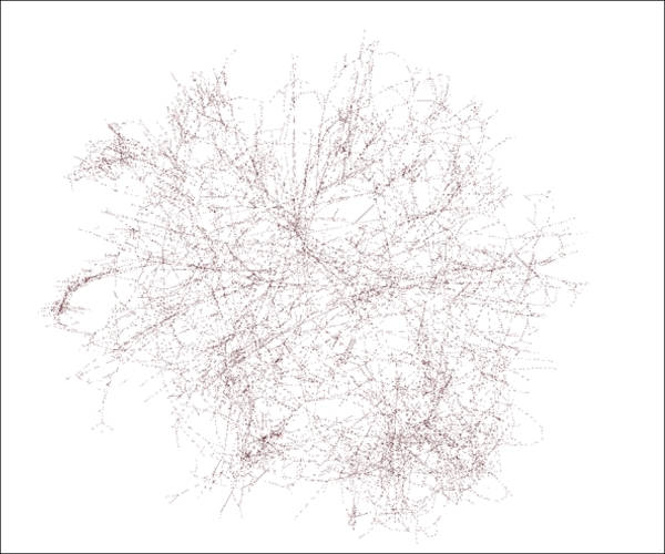
The Yifan Hu layout

Let your eyes scan the graph for a few moments to understand more about the network. Ready? Here are a few things you might have noticed:

Now let's use some automated approaches provided by Gephi to learn a bit more about this network. To begin this process, go to the Statistics tab in your Gephi workspace. Chapter 6, Graph Statistics, will provide additional details about a number of critical statistical functions, but for now, we'll get acquainted with a few of the common ones. Let's start with the Network Diameter option, as this provides three distinct measures that serve as important windows into every network's structure. Be sure to select the UnDirected option before you run your statistics.

The output screen gives you a few telling statistics, followed by some distribution graphs. This graph has a diameter of 46, which simply means that it would take 46 steps to traverse the graph between its two most distant points. This is a far cry from the notion of a small world graph, which is often known through the six degrees of separation term. Clearly, power grid networks are very different from social networks in structure. We also note an average path length just under 19; the typical node in this grid is about 19 steps away from any other point in the graph.

Scrolling down to the third graph (we'll bypass the first two for now; there's more in Chapter 6, Graph Statistics), we can see a very informative distribution on the eccentricity measure, which is shown by a bell-shaped curve. Eccentricity refers to the distance of a single point in the graph to its most distant point. Note that the minimum value here is 23, with very few nodes represented. These nodes can be thought of as being the most central within the structure of the network, as they require fewer steps to traverse the entire network. The mode value here is 33, with nearly 600 nodes requiring 33 steps to connect to the most distant point. Finally, the maximum value is 46, which is equivalent to the diameter of the network. These are the least central nodes in the structure and are very likely to be represented on the perimeter of most layouts.

Let's visit another simple statistic: Average Degree (we'll cover many more in Chapter 6, Graph Statistics). This measure will help any visual impressions we might already have about hubs and perhaps clustering by informing us about the typical number of neighbors per node. In this case, the answer is displayed via another distribution chart, where we can see that the overwhelming majority of nodes have either one, two, or three degrees, with an average of nearly 2.7. Again, we can contrast this with the familiar social network examples, where average degrees will often be in excess of 100.

For a final statistic, let's examine the clustering coefficients for this graph, which will give us a very clear indication of the graph density. The traditional clustering coefficient measured at the network level turns out to have a value of just 0.08, which means just eight percent of all possible graph triangles are complete. This indicates a graph that is not very dense. The average clustering coefficient, with more emphasis on local cliques, measures slightly higher at 0.107. In both cases, we confirm that the network is low density.

Now let's move on to the Filters tab, where some further network insight can be developed using a range of tools. Filtering is especially helpful when working with a dense graph, such as our power grid example; therefore, let's examine a couple of the most useful functions here with Chapter 5, Working with Filters, which is devoted to a deeper exploration of these capabilities. For these examples, go to the Topology folder within the Filters tab.

Assume that we want to focus on only the most highly connected nodes in the network, given that these points might serve as some sort of hub (albeit small ones in this network) with a high degree of importance. If we select the Degree Range option and drag it to the Queries portion of the tab, we see that nodes might have degrees ranging from a minimum of 1 to a maximum of 19. Using the slider bar and then clicking on the Filter button, we can then restrict the display to show only nodes with degrees of five and above, 10 and above, or whichever setting is selected. This can help dramatically reduce clutter in the graph and allow us to focus on the most important details while potentially identifying additional patterns in the network.

Next, we'll navigate to Attributes | Range and select the Eccentricity option. Recall our from earlier discovery that eccentricity values ranged between 23 and 46, with the most frequent value at 33. Let's suppose we wish to see only nodes with an eccentricity level below 30, representative of the nodes with the shortest paths across the network. Following the same process of dragging the Eccentricity attribute to the Queries space and then setting the maximum value to 30, we now see a graph with a greatly reduced number of nodes on display. If even more precision is needed, the maximum value can be set to 25, or any value of your choice, using either the slider bar or by manually entering a value.

Now that we have seen some of the basic functionalities with statistics and filters, it is time to move on to the process of modifying the graph for user consumption. The goal is to take actions to make the graph more navigable for users. Let's examine some of these actions in the next section.