
In my experience, selecting a perfect layout on the first attempt is highly unlikely; even if the best possible algorithm is chosen, it is almost a certainty that the graph display can be improved through adjusting the base settings, not to mention all of the downstream cosmetic enhancements. Knowing this makes it essential to sample multiple layouts for your network data, which can be a very efficient process for all but the largest networks.
In the next few sections, we will walk through the process of testing a few layouts using the same dataset, and will go into greater detail compared to our exercise in Chapter 2, A Network Graph Framework, by modifying settings within each algorithm to demonstrate the resulting impact on the network graph. We'll work with the Les Miserables dataset found in the Gephi samples (available when you open Gephi), as it provides an interesting network to work with, while still being small enough to easily interpret.
Our focus during this process will be limited to the actions that we can control primarily from the layout algorithms, in the hope that there will be sufficient differences that favor certain layouts over others. In later chapters, there will be a focus on additional modification that can be made once the base layout has been selected.
For this exercise, we will visit algorithms from several of the main categories discussed earlier—force-based, circular, and radial, and walk through a simple testing process. The goal is to not overwhelm you with image after image of each layout type, but rather to select a few layouts and then work within the layout to adjust settings and improve the graph appearance. This will be a nonjudgmental process as well, which will allow you to choose the layout that works best per your individual perception.
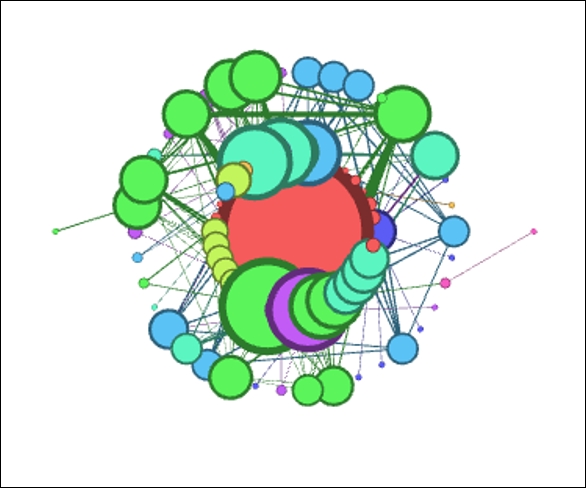
While there are many options for the force-directed layouts, the ARF algorithm provides a fast, simple, and easy to interpret layout that will aid in understanding the fundamentals of the force-based layouts. If you wish to follow along, use the Les Miserables dataset from the Gephi samples to get started. This is an undirected network that shows the interaction between characters in the famed novel.
Here's a look at what we see after opening the network in Gephi:
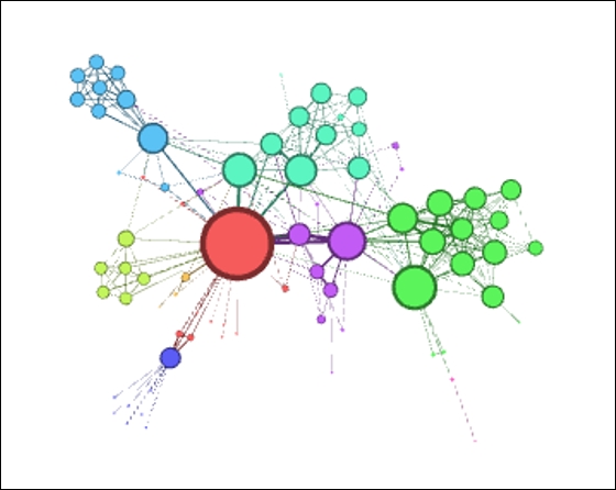
Les Miserables network from the .gexf format
Not bad as networks go—this one has obviously been worked on to some degree, with sized and colored nodes, weighted edges, and some sort of clustering tied into the colors. Still, we will work with our layout algorithms to see what improvements can be made.
Now, select the ARF layout if you choose to follow along (as you can recall, this must be installed as a plugin). Here are the default settings we'll use for the first iteration:
- Neighbor attraction force =
3.0 - General attraction force =
2.0 - Repulsive force =
8.0 - Precision =
2.0 - Maximum force =
7.0
Here is the result, after letting ARF run for about a minute:
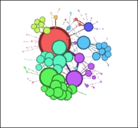
Les Miserables in ARF
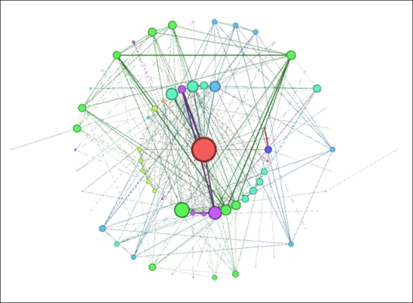
Notice that the network has actually drawn closer together compared to the original, making it more difficult to interpret. To remedy this, we'll adjust the repulsive force higher—say from 8.0 to 20.0, in an effort to spread the graph out by putting greater distance between unrelated nodes:
Les Miserables in ARF (Step 1)
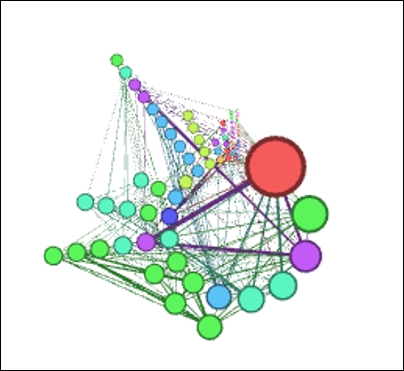
That's much better, although it still hasn't really surpassed the original, given that we have a few overlapping nodes that require attention. Let's give it one more try, this time adjusting the general attraction from 0.2 to 0.1. Reducing this value will minimize the likelihood that nodes are drawn together, thus preventing the overlapping (we hope!):
Les Miserables in ARF (Step 2)
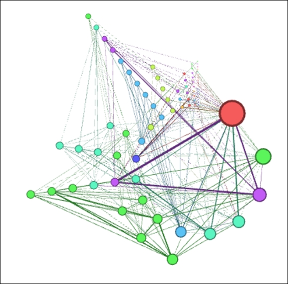
This is definitely an improvement over our first two attempts. The clustered nodes group together better than before, there are no overlaps, and peripheral characters have been pushed further toward the perimeter of the network, thus minimizing edge crossings and making for a cleaner layout. This final version feels like a good foundation we could take to subsequent stages in Gephi, assuming that we prefer the result versus the upcoming layouts we're about to view.
Our next effort will focus on the Concentric layout, available again as a Gephi plugin. The Les Miserables data provides an interesting use case for a concentric graph, given the dominance of a single character, Jean Valjean. If you are unfamiliar with the story, Valjean is the central character, and is thus represented by the largest node in the network, based on the number of connections to other characters. As you can recall from earlier, a single node is featured at the center of a concentric network, with other nodes spaced based on the number of degrees they are away from the selected node (for example, direct connections are represented in the innermost circle).
In theory, this would make a concentric layout an attractive option for telling this story, assuming that Valjean is at the center of our story. Let's have a look at whether this is as effective as it sounds. The default settings are as follows:
- Distance =
100 - Node =
0 - Speed =
10.0 - Coverage =
0.6
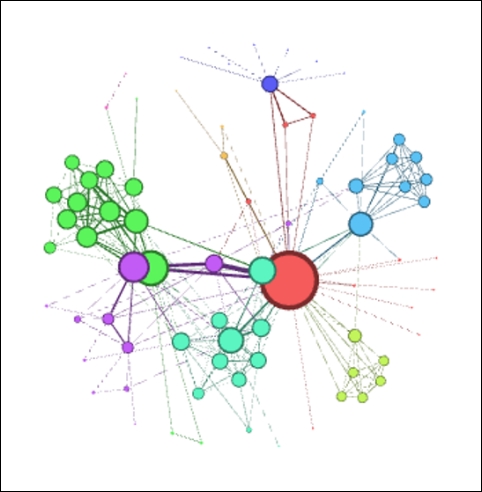
One change we do need to make is to set the node to Valjean's ID, which happens to be 11. Otherwise, the algorithm will do the selection for us, forcing an extra iteration to get things right. The initial result looks like this:
Les Miserables Concentric layout
These settings result in a very crowded graph that won't be effective in telling any sort of story. Perhaps if the nodes were not previously sized, this might work better, but we would then lose the impact conveyed by the multiple sizes. So let's increase the distance settings from 100 to 500 to spread the rings out from one another. Note that this is easily done given the small diameter of the network.
Les Miserables Concentric layout (Step 1)
Much improved! Now we can clearly see the structure of the network, and the fact that virtually all nodes are within two steps of the central character, with only a couple of instances three degrees out from the center. On the downside, the concentric approach isn't as effective in grouping the clusters compared to the ARF method, but at least it now presents a viable option for further use.
A Radial Axis layout resembles circular layouts to a considerable degree, but presents another option to consider that is different in one critical sense. The difference lies in the manner in which nodes are arranged and displayed using a series of axes rather than one or more circles. This would appear to be a reasonable approach for our current dataset, especially given the existing clusters in the network. Let's have a look at where this approach leads us, once again starting with default settings as follows:
- Scaling Width =
1.2 - Group Nodes by =
Degree
We'll leave the remainder of the settings untouched for now, although there are several more selections that could be used to tweak the layout. Here's the initial network graph:
Les Miserables Radial Axis
As with the other layout selections, the default settings have created a crowded graph, albeit somewhat more readable than our previous examples. Still, there are a couple of simple choices we can make to improve the layout quickly. Our first step, as with the other layouts, will be to spread the graph out for easier interpretation. Let's raise the Scaling Width option from 1.2 to 2.5 and see whether that level is sufficient for our purposes.
Les Miserables Radial Axis (Step 1)
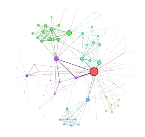
This is certainly an improvement, although a slightly higher setting might be even better, especially if we need to draw attention to some of the smaller nodes. For now, let's stick with this setting while making an important adjustment to the Group Nodes by option. Rather than using the default setting of Degrees, we're going to change this to group based on the clustered nodes, here shown as Modularity Class (Attribute). Let's check out the results of this change:
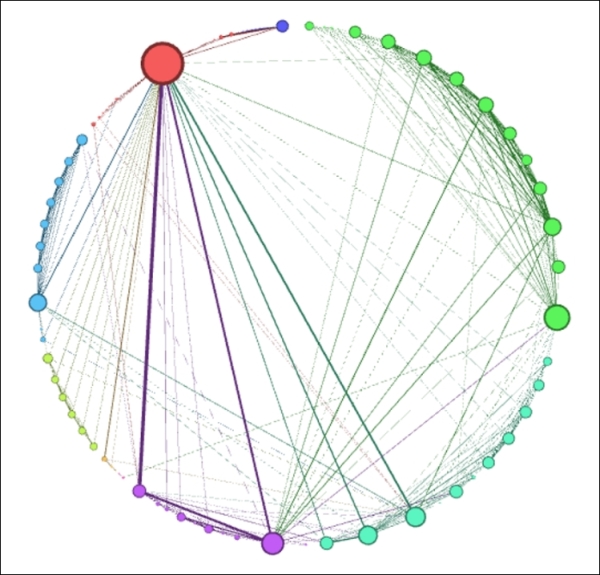
Les Miserables Radial Axis (Step 2)
Interesting—our Radial Axis layout has formed a circle, confirming our earlier statement about the similarities between circular and radial layouts. Also note how clean and easily followed the network is, with the various clusters ordered by size around the perimeter, and the Valjean node easily seen at the upper-left corner of the graph. This layout also highlights the strongest connections in the network, seen here through weighted edges between Valjean and some other prominent characters in the story.
While this layout worked quite well in this instance, note that it would probably be far less effective if we had 500 nodes rather than a mere 76 in this network. This is where your trained eye needs to make some decisions about how much is too much within a specific layout context, guided by how the network will ultimately be deployed.