Our first example showcasing tree-based methods in R will operate on a synthetic dataset that we have created. The dataset can be generated using commands in the companion R file for this chapter, available from the publisher. The data consists of 287 observations of two input features, x1 and x2.

The output variable is a categorical variable with three possible classes: a, b, and c. If we follow the commands in the code file, we will end up with a data frame in R, mcdf:

> head(mcdf, n = 5)
          x1       x2 class
1 18.58213 12.03106     a
2 22.09922 12.36358     a
3 11.78412 12.75122     a
4 23.41888 13.89088     a
5 16.37667 10.32308     a

This problem is actually very simple because, on the one hand, we have a very small dataset with only two features, and on the other the classes happen to be quite well separated in the feature space, something that is very rare. Nonetheless, our objective in this section is to demonstrate the construction of a classification tree on well-behaved data before we get our hands (or keyboards) dirty on a real-world dataset in the next section.

To build a classification tree for this dataset, we will use the tree package, which provides us with the tree() function that trains a model using the CART methodology. As is the norm, the first parameter to be provided is a formula and the second parameter is the data frame. The function also has a split parameter that identifies the criterion to be used for splitting. By default, this is set to deviance for the deviance criterion, for which we observed better performance on this dataset. We encourage readers to repeat these experiments by setting the split parameter to gini for splitting on the Gini index.

Without further ado, let us train our first decision tree:

> library(tree)
> d2tree <- tree(class ~ ., data = mcdf)
> summary(d2tree)

Classification tree:
tree(formula = class ~ ., data = mcdf)
Number of leaf nodes:  5 
Residual mean deviance:  0.03491 = 9.844 / 282 
Misclassification error rate: 0.003484 = 1 / 287

We invoke the summary() function on our trained model to get some useful information about the tree we built. Note that for this example, we won't be splitting our data into a training and test set, as our goal is to discuss the quality of the model fit first. From the provided summary, we seem to have only misclassified a single example in our entire dataset. Ordinarily, this would raise suspicion that we are overfitting; however, we already know that our classes are well separated in the feature space. We can use the plot() function to plot the shape of our tree as well as the text() function to display all the relevant labels so we can fully visualize the classifier we have built:

> plot(d2tree)
> text(d2tree, all = T)

This is the plot that is produced:

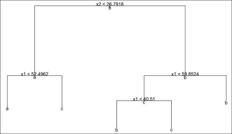
Note that our plot shows a predicted class for every node, including non-leaf nodes. This simply allows us to see which class is predominant at every step of the tree. For example, at the root node, we see that the predominant class is class b, simply because this is the most commonly represented class in our dataset. It is instructive to be able to see the partitioning of our 2D space that our decision tree represents.

For one and two features, the tree package allows us to use the partition.tree() function to visualize our decision tree. We have done this and superimposed our original data over it in order to see how the classifier has partitioned the space:

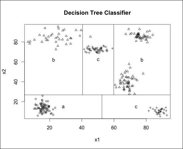
Most of us would probably identify six clusters in our data; however, the clusters on the top-right of the plot are both assigned to class b and so the tree classifier has identified this entire region of space as a single leaf node. Finally, we can spot the misclassified point belonging to class b that has been assigned to class c (it is the triangle in the middle of the top part of the graph).

Another interesting observation to make is how efficiently the space has been partitioned into rectangles in this particular case (only five rectangles for a dataset with six clusters). On the other hand, we can expect this model to have some instabilities because several of the boundaries of the rectangles are very close to data points in the dataset (and thus close to the edges of a cluster). Consequently, we should also expect to obtain a lower accuracy with unseen data that is generated from the same process that generated our training data.

In the next section, we will build a tree model for a real-world classification problem.