Chapter 14: Solving Robot Learning

So far in the book, we have covered many state-of-the-art algorithms and approaches in reinforcement learning. Now, starting with this chapter, we will see them in action to take on real-world problems! We start with robot learning, an important application area for reinforcement learning. To this end, we will train a Kuka robot to grasp objects on a tray using PyBullet physics simulation. We will discuss several ways of solving this hard-exploration problem and solve it both using a manually crafted curriculum as well as using the ALP-GMM algorithm. At the end of the chapter, we will present other simulation libraries for robotics and autonomous driving, which are commonly used to train reinforcement learning agents.

So, this chapter covers:

• Introducing PyBullet
• Getting familiar with the Kuka environment
• Developing strategies to solve the Kuka environment
• Using curriculum learning to train the Kuka robot
• Going beyond PyBullet, into autonomous driving

This is one of the most challenging and fun areas for reinforcement learning. Let's dive right in!

Introducing PyBullet

PyBullet is a popular high-fidelity physics simulation for robotics, machine learning, games, and more. It is one of the most commonly used libraries for robot learning using RL, especially in sim-to-real transfer research and applications.

Figure 14.1 – PyBullet environments and visualizations (source: PyBullet GitHub repo)

PyBullet allows developers to create their own physics simulations. In addition, it has prebuilt environments using the OpenAI Gym interface. Some of those environments are shown in Figure 14.1.

In the next section, we will set up a virtual environment for PyBullet.

Setting up PyBullet

It is almost always a good idea to work in virtual environments for Python projects, which is also what we do for our robot learning experiments in this chapter. So, let's go ahead and execute the following commands to install the libraries we will use:

$ virtualenv pybenv

$ source pybenv/bin/activate

$ pip install pybullet --upgrade

$ pip install gym

$ pip install tensorflow==2.3.1

$ pip install ray[rllib]==1.0.0

$ pip install scikit-learn==0.23.2

You can test whether your installation is working by running:

$ python -m pybullet_envs.examples.enjoy_TF_AntBulletEnv_v0_2017may

And if everything is working fine, you will see a cool Ant robot wandering around as in Figure 14.2.

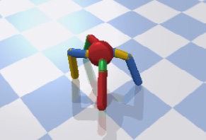
Figure 14.2 – Ant robot walking in PyBullet

Great! We are now ready to proceed to the Kuka environment that we will use.

Getting familiar with the Kuka environment

KUKA is a company that offers industrial robotics solutions, which are widely used in manufacturing and assembly environments. PyBullet includes a simulation of a KUKA robot, used for object grasping simulations (Figure 14.3).

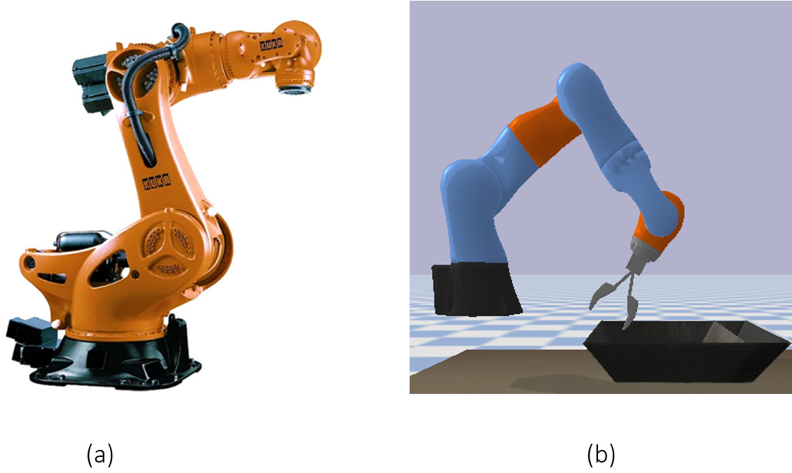
Figure 14.3 – KUKA robots are widely used in industry. (a) A real KUKA robot (image source CNC Robotics website), (b) a PyBullet simulation.

There are multiple Kuka environments in PyBullet for:

• Grasping a rectangle block using robot and object position and angles,
• Grasping a rectangle block using camera inputs,
• Grasping random objects using camera/position inputs.

In this chapter, we focus on the first one, which we look into next in more detail.

Grasping a rectangle block using a Kuka robot

In this environment, the goal of the robot is to reach a rectangle object, grasp it, and raise it up to a certain height. An example scene from the environment, along with the robot coordinate system, are shown in Figure 14.4.

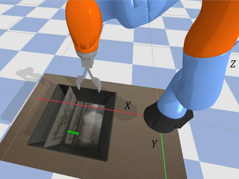
Figure 14.4 – Object grasping scene and the robot coordinate system

The dynamics and initial position of the robot joints are defined in the Kuka class of the pybullet_envs package. We will talk about these details only as much as we need to, but you should feel free to dive into the class definition to better understand the dynamics.

Info

To better understand the PyBullet environment and how the Kuka class is constructed, you can check out the PyBullet Quickstart Guide at https://bit.ly/323PjmO.

Let's now dive into the Gym environment created to control this robot inside PyBullet.

Kuka Gym environment

The KukaGymEnv wraps the Kuka robot class and turns it into a Gym environment. The action, observation, reward and terminal conditions are defined as below.

Actions

There are three types of actions the agent takes in the environment, which are all about moving the gripper. These actions are:

• Velocity along the axis,
• Velocity along the axis,
• Angular velocity to rotate the gripper (yaw).

The environment itself moves the gripper along the axis towards the tray, where the object is located. When it gets sufficiently close to the tray, it closes the fingers of the gripper to try grasping the object.

The environment can be configured to accept discrete or continuous actions. We will use the latter in our case.

Observations

The agent receives 9 observations from the environment:

• Three observations for the , , and positions of the gripper,
• Three observations for the Euler angles of the gripper with respect to the , , and axes,
• Two observations for the and positions of the object relative to the gripper,
• One observation for the Euler angle of the object relative to the gripper's Euler angle along the axis.

Reward

The reward for grasping the object successfully and lifting it up to a certain height is 10,000 points. Other than that, there is a slight cost that penalizes the distance between the gripper and the object. Additionally, there is also some energy cost for rotating the gripper.

Terminal conditions

An episode terminates after 1000 steps or when the after the gripper closes, whichever occurs first.

The best way to wrap your mind around how the environment works is actually experiment with it, which you can do next using the following code: Chapter14/manual_control_kuka.py

This script allows you to control the robot manually. You can use the "gym-like" control mode, where the vertical speed and the gripper finger angles are controlled by the environment. Alternatively, you can choose the non-gym-like mode to exert more control.

One thing you will notice that even if you keep the speeds along the and axes zero, in the gym-like control mode, the robot will change its and positions while going down. This is because the default speed of the gripper along the axis is too high. You can actually verify that in the non-gym-like mode: Values below for alter the positions on the other axes too much. We will reduce the speed when we customize the environment to alleviate that.

Now that you are familiar with the Kuka environment, let's discuss some alternative strategies to solve it.

Developing strategies to solve the Kuka environment

The object grasping problem in the environment is a hard-exploration problem, meaning that it is unlikely to stumble upon the sparse reward that the agent receives at the end upon grasping the object. Reducing the vertical speed as we will do will make is a bit easier. Still, let's refresh our minds about what strategies we have covered to address these kinds of problems:

• Reward shaping is one of the most common machine teaching strategies that we discussed earlier. In some problems, incentivizing the agent towards the goal is very straightforward. In many problems, though, it can be quite painful. So, unless there is an obvious way of doing so, crafting the reward function may just take too much time (and expertise about the problem). Also notice that the original reward function has a component to penalize the distance between the gripper and the object, so the reward is already shaped to some extent. We will not go beyond that in our solution.
• Curiosity-driven learning incentivizes the agent for discovering new parts of the state space. For this problem, though, we don't need the agent to randomly explore the state space too much as we have already some idea about what it should do. So, we will skip this technique as well.
• Increasing the entropy of the policy incentivizes the agent to diversify its actions. The coefficient for this can be set using the "entropy_coeff" config inside the PPO trainer of RLlib, which is what we will use. However, our hyperparameter search (we will come to it soon) ended up picking this value as zero.
• Curriculum learning is perhaps the most suitable approach here. We can identify what makes the problem challenging for the agent, start training it at easy levels, and gradually increase the difficulty.

So, curriculum learning is what we will leverage to solve this problem. But first, let's identify the dimensions to parametrize the environment to create a curriculum.

Parametrizing the difficulty of the problem

When you experimented with the environment, you may have noticed the factors that make the problem difficult:

• The gripper starts too high to discover the correct sequences of actions to grasp the object. So, the robot joint that adjusts the height will be one dimension we will parameterize. It turns out that this is set in the second element of the jointPositions array of the Kuka class.
• When the gripper is not at its original height, it may get misaligned with the location of the object along the axis. We will also parametrize the position of the joint that controls this, which is the fourth element of the jointPositions array of the Kuka class.
• Randomizing the object position is another source of difficulty for the agent, which takes place for the and positions as well as the object angle. We will parametrize the degree of randomization between 0 and 100% for each of these components.
• Even when the object is not randomly positioned, its center is not aligned with the default position of the robot on the axis. We will add some bias to the position of the object, again parametrized.

This is great! We know what to do, which is a big first step. Now, we can go into curriculum learning!

Using curriculum learning to train the Kuka robot

The first step before actually kicking off some training is to customize the Kuka class as well as the KukaGymEnv to make them work with the curriculum learning parameters we described above. So, let's do that next.

Customizing the environment for curriculum learning

First, we start with creating a CustomKuka class which inherits the original Kuka class of PyBullet. Here is how we do it:

Chapter14/custom_kuka.py

1. We first need to create the new class, and accept an additional argument, jp_override dictionary, which stands for joint position override.

   class CustomKuka(Kuka):

       def __init__(self, *args,

                    jp_override=None, **kwargs):

           self.jp_override = jp_override

           super(CustomKuka, self).__init__(*args, **kwargs)

2. We need this to change the jointPositions array set in the reset method.

       def reset(self):

       ...

           if self.jp_override:

               for j, v in self.jp_override.items():

                   j_ix = int(j) - 1

                   if j_ix >= 0 and j_ix <= 13:

                       self.jointPositions[j_ix] = v

   Now, it's time to create CustomKukaEnv.

3. Create the custom environment that accepts all these parametrization inputs for curriculum learning.

   class CustomKukaEnv(KukaGymEnv):

       def __init__(self, env_config={}):

           renders = env_config.get("renders", False)

           isDiscrete = env_config.get("isDiscrete", False)

           maxSteps = env_config.get("maxSteps", 2000)

           self.rnd_obj_x = env_config.get("rnd_obj_x", 1)

           self.rnd_obj_y = env_config.get("rnd_obj_y", 1)

           self.rnd_obj_ang = env_config.get("rnd_obj_ang",

                                             1)

           self.bias_obj_x = env_config.get("bias_obj_x", 0)

           self.bias_obj_y = env_config.get("bias_obj_y", 0)

           self.bias_obj_ang =

                          env_config.get("bias_obj_ang", 0)

           self.jp_override = env_config.get("jp_override")

           super(CustomKukaEnv, self).__init__(

                                      renders=renders,

                                      isDiscrete=isDiscrete,

                                      maxSteps=maxSteps)

   Note that we are also making it RLlib compatible by accepting an env_config.

4. We use the randomization parameters in the reset method to override the default amount of randomization in the object position.

       def reset(self):

           ...

           xpos = 0.55 + self.bias_obj_x +

                  0.12 * random.random() * self.rnd_obj_x

           ypos = 0 + self.bias_obj_y + 0.2 *

                  random.random() * self.rnd_obj_y

           ang = (

               3.14 * 0.5

               + self.bias_obj_ang

               + 3.1415925438 * random.random() *

                 self.rnd_obj_ang)

5. Also, we should now replace the old Kuka class with CustomKuka and pass the joint position override input to it.

           ...

           self._kuka = CustomKuka(

               jp_override=self.jp_override,

               urdfRootPath=self._urdfRoot,

               timeStep=self._timeStep)

6. Finally, we override the step method of the environment to decrease the default speed on the axis.

       def step(self, action):

           dz = -0.0005

           ...

   ...

               realAction = [dx, dy, dz, da, f]

           obs, reward, done, info = self.step2(realAction)

           return obs, reward / 1000, done, info

   Also notice that we rescaled the reward (it will end up between -10 and 10) to make the training easy.

Great job! Next, let's discuss what kind of curriculum to use.

Designing the lessons in the curriculum

It is one thing to determine the dimensions to parametrize the difficulty of the problem, and another thing to decide how to expose this parametrization to the agent. We know that the agent should start with easy lessons and move to more difficult ones gradually. This, though, raises some important questions:

• Which parts of the parametrized space are easy?
• What should be the step sizes to change the parameters between lesson transitions? In other words, how should we slice the space into lessons?
• What are the criteria of success for the agent to transition to a next lesson?
• What if the agent fails in a lesson, meaning that its performance is unexpectedly bad? Should it go back to the previous lesson? What is the bar for failure?
• What if the agent cannot transition into the next lesson for a long time? Does it mean that we set the bar for success for the lesson too high? Should we divide that lesson into sub-lessons?

As you can see, these are non-trivial questions to answer when we are designing a curriculum manually. But also remember that in Chapter 11, Achieving Generalization and Overcoming Partial Observability, we introduced the Absolute Learning Progress with Gaussian Mixture Models (ALP-GMM) method, which handles all these decisions for us. Here, we will implement both, starting with a manual curriculum first.

Training the agent using a manually designed curriculum

We will design a rather simple curriculum for this problem. It will transition the agent to subsequent lessons when it meets the success criteria, without falling back to a previous lesson in case of low performance. The curriculum will be implemented as a method inside the CustomKukaEnv class, using the increase_difficulty method:

1. We start by defining the delta changes in the parameter values during lesson transitions. For the joint values, we will decrease the joint positions from what is entered by the user (easy) to the original values in the environment (difficult).

       def increase_difficulty(self):

           deltas = {"2": 0.1, "4": 0.1}

           original_values = {"2": 0.413184, "4": -1.589317}

           all_at_original_values = True

           for j in deltas:

               if j in self.jp_override:

                   d = deltas[j]

                   self.jp_override[j] =

            max(self.jp_override[j] - d, original_values[j])

                   if self.jp_override[j] !=

            original_values[j]:

                       all_at_original_values = False

2. During each lesson transition, we also make sure to increase the randomization of the object position.

           self.rnd_obj_x = min(self.rnd_obj_x + 0.05, 1)

           self.rnd_obj_y = min(self.rnd_obj_y + 0.05, 1)

           self.rnd_obj_ang = min(self.rnd_obj_ang + 0.05,

                                  1)

3. Finally, we remember to set the biases to zeros when the object position becomes fully randomized:

           if self.rnd_obj_x == self.rnd_obj_y ==

                                self.rnd_obj_ang == 1:

               if all_at_original_values:

                   self.bias_obj_x = 0

                   self.bias_obj_y = 0

                   self.bias_obj_ang = 0

So far so good, we have almost everything ready to train our agent. One last thing before doing so, let's discuss how to pick the hyperparameters.

Hyperparameter selection

In order to tune the hyperparameters in RLlib, we can use Ray's Tune library. In Chapter 15, Supply Chain Management, we will provide you with an example of how it is done. For now, you can just use the hyperparameters we have picked in Chapter14/configs.py.

Tip

In hard-exploration problems, it may make more sense to tune the hyperparameters for a simple version of the problem. This is because without observing some reasonable rewards, the tuning may not pick a good set of hyperparameter values. After we do an initial tuning in an easy environment setting, some of the chosen values can be adjusted later in the process if the learning stalls.

Finally, let's see how we can use the environment we have just created during training with the curriculum we have defined.

Training the agent on the curriculum using RLlib

To proceed with the training, we need the following ingredients:

• Initial parameters for the curriculum,
• Some criteria to define the success (and failure, if needed),
• A callback function that will execute the lesson transitions.

In the code snippet below, we use the PPO algorithm in RLlib, set the initial parameters, and set the reward threshold to 5.5 (empirically determined, feel free to try other values) in the callback function that executes the lesson transitions.

Chapter14/train_ppo_manual_curriculum.py

config["env_config"] = {

    "jp_override": {"2": 1.3, "4": -1}, "rnd_obj_x": 0,

    "rnd_obj_y": 0, "rnd_obj_ang": 0, "bias_obj_y": 0.04}

def on_train_result(info):

    result = info["result"]

    if result["episode_reward_mean"] > 5.5:

        trainer = info["trainer"]

        trainer.workers.foreach_worker(

            lambda ev: ev.foreach_env(lambda env:

                          env.increase_difficulty()))

ray.init()

tune.run("PPO", config=dict(config,

                **{"env": CustomKukaEnv,

                   "callbacks": {

                    "on_train_result": on_train_result}}

                      ),

          checkpoint_freq=10)

This should kick off the training and you will see the curriculum learning in action! You will notice that as the agent transitions to a next lesson, its performance will drop suddenly once in a while as the environment gets more difficult with lesson transitions.

We will look into the results from this training later. Let's now also implement the ALP-GMM algorithm.

Curriculum learning using absolute learning progress

The ALP-GMM method focuses on where the biggest performance change (absolute learning progress) in the parameter space is and generates parameters around that gap. This idea is illustrated in Figure 14.5.

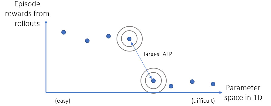
Figure 14.5 – ALP-GMM generates parameters (tasks) around points, between which the biggest episode reward change is observed.

This way, the learning budget is not spent on the parts of the state space that has already been learned, or on the parts that are too difficult to learn for the current agent, but where the agent can take on more difficulties without being overwhelmed.

After this recap, let's go ahead and implement it. We start with creating a custom environment in which the ALP-GMM algorithm will run.

Chapter14/custom_kuka.py

We get the ALP-GMM implementation directly from the source repo accompanying the paper (Portelas et al. 2019) and put it under Chapter14/alp. We can then plug that into the new environment we create, ALPKukaEnv, the key pieces of which are below:

1. We create the class and define all the minimum and maximum values of the parameter space we are trying to teach the agent.

   class ALPKukaEnv(CustomKukaEnv):

       def __init__(self, env_config={}):

           ...

           self.mins = [...]

           self.maxs =  [...]

           self.alp = ALPGMM(mins=self.mins,

                        maxs=self.maxs,

                              params={"fit_rate": 20})

           self.task = None

           self.last_episode_reward = None

           self.episode_reward = 0

           super(ALPKukaEnv, self).__init__(env_config)

   Here, the task is the latest sample from the parameter space generated by the ALP-GMM algorithm to configure the environment.

2. A task is sampled at the beginning of each episode. Once an episode finishes, the task (environment parameters used in the episode) and the episode reward are used to update the GMM model.

       def reset(self):

           if self.task is not None and

              self.last_episode_reward is not None:

               self.alp.update(self.task,

                               self.last_episode_reward)

           self.task = self.alp.sample_task()

           self.rnd_obj_x = self.task[0]

           self.rnd_obj_y = self.task[1]

           self.rnd_obj_ang = self.task[2]

           self.jp_override = {"2": self.task[3],

                               "4": self.task[4]}

           self.bias_obj_y = self.task[5]

           return super(ALPKukaEnv, self).reset()

3. And finally, we make sure to keep track of the episode reward:

       def step(self, action):

           obs, reward, done, info = super(ALPKukaEnv,

                                     self).step(action)

           self.episode_reward += reward

           if done:

               self.last_episode_reward =

                         self.episode_reward

               self.episode_reward = 0

           return obs, reward, done, info

One thing to note here is that ALP-GMM is normally implemented in a centralized fashion: A central process generates all the tasks for the rollout workers and collects the episode rewards associated with those tasks to process. Here, since we are working in RLlib, it is easier to implemented it inside the environment instances. In order to account for the reduced amount of data collected in a single rollout, we used "fit_rate": 20, lower from the original level of 250, so that a rollout worker doesn't wait too long before it fits a GMM to the task-reward data it collects.

After creating the ALPKukaEnv, the rest is just a simple call of Ray's tune.run() function, which is available in Chapter14/train_ppo_alp.py. Note that, unlike in a manual curriculum, we don't specify the initial values of the parameters. Instead, we have passed their bounds the ALP-GMM processes, which guide the curriculum within those bounds.

Now, we are ready to do a curriculum learning bake off!

Comparing the experiment results

We kick off three training sessions using the manual curriculum we described, the ALP-GMM, and one without any curriculum implemented. The TensorBoard view of the training progresses is shown in Figure 14.6:

Figure 14.6 – Training progresses on TensorBoard

A first glance might tell you that the manual curriculum and ALP-GMM are close, while not using a curriculum is a distant third. Actually, this is not the case. Let's unpack this plot:

• Manual curriculum goes from easy to difficult, that is why it is at the top, most of the time. In our run, it could not even get to the latest lesson within the time budget. Therefore, the performance shown in the figure is inflated for the manual curriculum.
• The no-curriculum training is always competing at the most difficult level. That is why it is at the bottom most of the time: The other agents are not running against the hardest parameter configurations as they slowly get there.
• ALP-GMM is in the middle for the most part, because it is experimenting with difficult and hard configurations at the same time, while focusing on somewhere in between.

  Since this plot is inconclusive, we evaluate the agents on the original (most difficult) configuration. The results are the following after 100 test episodes for each:

  Agent ALP-GMM score: 3.71

  Agent Manual score: -2.79

  Agent No Curriculum score: 2.81

• The manual curriculum performed the worst as it could not get to the latest lesson as of the end of the training.
• The no-curriculum had some success, but starting with the most difficult setting seems to have set it back. Also, the evaluation performance is in line with what is shown on TensorBoard, since the evaluation settings are no different from the training settings in this case.
• ALP-GMM seems to have benefited from gradually increasing the difficulty and performs the best.
• The no-curriculum training's peak point in the TensorBoard graph is similar to the ALP-GMM's latest performance. So, our modification with respect to the vertical speed of the robot diminished the difference between the two. Not using a curriculum, however, causes the agent to not learn at all in many hard-exploration scenarios.

You can find the code for the evaluation in Chapter14/evaluate_ppo.py. Also, you can use the script Chapter14/visualize_policy.py to watch your trained agents in action, see where they fall short and come up with ideas to improve the performance!

This concludes our discussion on the Kuka example of robot learning. In the next section, we will wrap up this chapter with a list of some popular simulation environments used in training autonomous robots and vehicles.

Going beyond PyBullet into autonomous driving

PyBullet is a great environment to test the capabilities of reinforcement learning algorithms in a high-fidelity physics simulation. Some of the other libraries you will come across at the intersection of robotics and reinforcement learning are:

• Gazebo: http://gazebosim.org/,
• MuJoCo (requires license): http://www.mujoco.org/,
• Adroit: https://github.com/vikashplus/Adroit.

In addition, you will also see Unity and Unreal Engine-based environments used in training reinforcement learning agents.

The next and more popular level of autonomy is of course autonomous vehicles. RL is increasingly experimented in realistic autonomous vehicle simulations as well. The most popular libraries in this area are:

• CARLA: https://github.com/carla-simulator/carla,
• AirSim: https://github.com/microsoft/AirSim. (Disclaimer: The author is a Microsoft employee at the time of authoring this book and part of the organization developing AirSim.)

With this, we conclude this chapter on robot learning. This is a very hot application area in RL, and there are many environments you can experiment with. I hope you have enjoyed and are inspired by what we have done in this chapter.

Summary

Autonomous robots and vehicles are going to play a huge role in the future of our world; and reinforcement learning is one of the primary approaches to create such autonomous systems. In this chapter, we have taken a peek at what it looks like to train a robot to accomplish an object grasping task, a major challenge in robotics with many applications in manufacturing and warehouse material handling. We used the PyBullet physics simulator to train a Kuka robot in a hard-exploration setting, for which we leveraged both manual and ALP-GMM-based curriculum learning. Now that you have a fairly good grasp of how to utilize these techniques, you can take on other similar problems.

In the next chapter, we will look into another major area for reinforcement learning applications: Supply chain management. Stay tuned for another exciting journey!

References

1. Coumans, E., Bai, Y. (2016-2019). PyBullet, a Python module for physics simulation for games, robotics and machine learning. URL: http://pybullet.org.
2. Bulletphysics/Bullet3. (2020). Bullet Physics SDK, GitHub. URL: https://github.com/bulletphysics/bullet3.
3. CNC Robotics. (2018). KUKA Industrial Robots, Robotic Specialists. URL: https://www.cncrobotics.co.uk/news/kuka-robots/.
4. KUKA AG. (2020). URL: https://www.kuka.com/en-us.
5. Portelas, Rémy, et al. (2019). Teacher Algorithms for Curriculum Learning of Deep RL in Continuously Parameterized Environments. ArXiv:1910.07224 [Cs, Stat], Oct. 2019. arXiv.org, http://arxiv.org/abs/1910.07224.
6. Gonnochenko, Aleksei, et al. (2020). Coinbot: Intelligent Robotic Coin Bag Manipulation Using Deep Reinforcement Learning and Machine Teaching. arXiv.org, http://arxiv.org/abs/2012.01356.