Search in book...
Toggle Font Controls
Create new playlist

Name your new playlist

Playlist description (optional)
Sign In

Email address

Password

Forgot Password?

or

Continue with Facebook

Continue with Google
Sign Up

Full Name

Email address

Confirm Email Address

Password

or

Continue with Facebook

Continue with Google

Chapter 8

Curves

8.1 Introduction

Curves form the backbone of geometric modeling to create solid models. A sketch consists of multiple curves that are connected to form closed contours (loops). Loops may be nested. A sketch that consists of only one contour generates a solid without holes, whereas a sketch with multiple contours generates a solid with holes in it. Figure 8.1 shows examples. Figure 8.1A shows a one-contour sketch. You can create a sketch with only one-level nesting (i.e., an outside contour with one or more disconnected contours inside it), as shown in Figure 8.1B. However, if you attempt to use more than one-level nesting, as shown in Figure 8.1C, the solid creation operation fails.

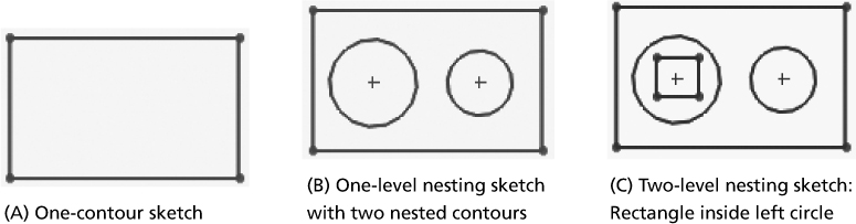
Three figures show different types of nesting contours. — **Figure 8.1** Nesting contours to create solids

Mathematically, two families of curves exist. The first family is analytic curves, which have closed-form equations defining them. Examples of analytic curves include lines, circles, ellipses, parabolas, and hyperbolas. This family is also known as conics because the curves result from intersecting a cone with a plane. For example, intersecting a cone with a plane passing through its axis produces a line. Intersecting a cone with a plane perpendicular to its axis produces a circle; and, if the plane is not perpendicular to the cone, the intersection results in an ellipse, a parabola, or a hyperbola.

The second family of curves is synthetic curves. A synthetic curve is defined by a polynomial that uses a set of data points. These data points control the curve shape. Examples include a cubic curve and a B-spline (or a spline, as SolidWorks calls it). Figure 8.2 shows the curves in the SolidWorks menus. These curves are accessible from the SolidWorks Sketch tab. The ellipse is defined by two radii (each connecting two opposite points, as shown in Figure 8.2A), and the spline is defined by points P₀, P₁, ..., P _n.

A figure shows the curves present in the SolidWorks menu. — **Figure 8.2** Families of curves

Synthetic curves offer more flexibility in modeling than do analytic curves. They are efficient to use for creating free-form shapes. All you need to do is define the curve points by either clicking in the sketch area or entering (x, y, z) coordinates. After a curve is created, you can easily modify its shape by editing its points to change their locations.

8.2 Curve Representation

Curves and surfaces can be described mathematically by nonparametric (explicit) or parametric equations. A point on a curve has (x, y) coordinates for planar (sketch) curves, and (x, y, z) coordinates for nonplanar curves. For a planar curve, an explicit equation relates the y coordinate to the x coordinate as follows:

\begin{matrix} y = f (x) x_{\min} \leq x \leq x_{\max} & (8.1) \end{matrix}

Explicit equations for nonplanar curves are complex and are not supported by CAD/CAM systems because they do not lend themselves well to the CAD design environment.

A parametric equation is an equation that uses a parameter (e.g., u) to describe the (x, y) coordinates of a point on a planar curve or the (x, y, z) coordinates of a point on a nonplanar curve. Figure 8.3 shows the parametric representation of a curve. The parameter u starts with a minimum value, u _min, at one end of the curve and finishes with a maximum value, u _max, at the other end of the curve. The parameter increases in value from u _min to u _max, thus defining the parameterization direction of the curve as indicated by the arrow on the curve. Any point P on the curve is defined by its position vector, P, that is a function of u:

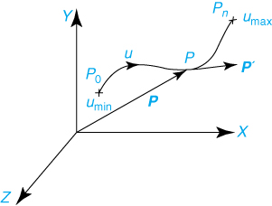
A curve u rising from P 0 at u min to a straight line at point P and again rises as a curve to P n at u max . A vector extends to P from the origin. — **Figure 8.3** Parametric curve

\begin{matrix} P = P (u) u_{\min} \leq u \leq u_{\max} & (8.2) \end{matrix}

Alternatively, point P is defined by its (x, y, z) coordinates. Thus:

\begin{matrix} P = [\begin{array}{l} x \\ y \\ z \end{array}] = [\begin{array}{l} x (u) \\ y (u) \\ z (u) \end{array}] u_{\min} \leq u \leq u_{\max} & (8.3) \end{matrix}

The tangent vector P ' at any point on the curve (Figure 8.3) is given by:

\begin{matrix} P' = \frac{d P}{d u} = [\begin{array}{l} x' \\ y' \\ z' \end{array}] u_{\min} \leq u \leq u_{\max} & (8.4) \end{matrix}

The tangent vector is an important concept in CAD/CAM applications such as mass property calculations and NC (numerical control) programming. For these two applications, you use the tangent vector at any point on the curve to calculate the normal vector to the curve at the same point. For mass properties, the direction of the normal vector is used to determine the inside (where material is) and the outside (where holes exist) of the solid. For NC programming, you move the cutting tool along the direction of the normal vector until it makes contact with the part surface to be machined. This minimizes the lateral (shear) forces on the cutting tool, which in turn reduces the chance of breaking the tool when it comes in contact with the surface to be machined.

SolidWorks supports both explicit and parametric equations for curves. It allows the user to enter explicit equations for planar (sketch) curves. It does not support explicit equations for nonplanar curves. However, it does support parametric equations for both planar and nonplanar curves. It uses the parameter t instead of u. This chapter shows how to enter and use equations in SolidWorks.

8.3 Line Parametric Equation

Figure 8.4 shows the parametric representation of a straight line defined by two endpoints, P₀ and P₁. The parameterization direction of the line shown in Figure 8.4 goes from P₀ to P₁, indicating that you start sketching the line at P₀ and finish at P₁. The parametric equation of this line is given (in vector form) by:

\begin{matrix} P = P (u) = P_{0} + u (P_{1} - P_{0}) 0 \leq u \leq 1 & (8.5) \end{matrix}

A line u rising from P 0 at u = 0 through point P till P 1 at u = 1. A vector extends to P from the origin. — **Figure 8.4** Parametric line

or, in scalar form:

\begin{matrix} P = P (u) = [\begin{array}{l} x (u) \\ y (u) \\ z (u) \end{array}] = [\begin{array}{l} x_{0} + u (x_{1} - x_{0}) \\ y_{0} + u (y_{1} - y_{0}) \\ z_{0} + u (z_{1} - z_{0}) \end{array}] 0 \leq u \leq 1 & (8.6) \end{matrix}

Using Eq. (8.4), the tangent vector of the line is given by:

\begin{matrix} P' = [\begin{array}{l} x' \\ y' \\ z' \end{array}] = [\begin{array}{l} x_{1} - x_{0} \\ y_{1} - y_{0} \\ z_{1} - z_{0} \end{array}] & (8.7) \end{matrix}

Eq. (8.7) shows that the tangent vector is constant (independent of u), as expected. You can easily derive the line slope from the tangent vector. For example, the line slope in the XY plane is given by:

\begin{matrix} \frac{d y}{d x} = \frac{d y / d u}{d x / d u} = \frac{y ​ ​'}{x'} & (8.8) \end{matrix}

The elegance of the parametric representation is that it is independent of the dimensionality of the modeling space, whether it is 2D (x and y coordinates only) or 3D (x, y, and z coordinates). In other words, use z = 0 in the 3D equations, and you get 2D modeling. As a matter of fact, when you sketch in a sketch plane, the z value is set to 0; when you are done sketching, SolidWorks transforms the sketch 2D WCS coordinates to 3D MCS coordinates.

8.4 Circle Parametric Equation

In this section, we consider the case of a circle defined by a center point (x_c, y_c) and a radius R only to simplify the formulation. When you sketch a circle, you must define a sketch plane because a center and a radius define an infinite number of circles. Figure 8.5 shows this definition of a parametric circle. The parameter u is the angle, measured in counterclockwise direction. The circle equation is given by:

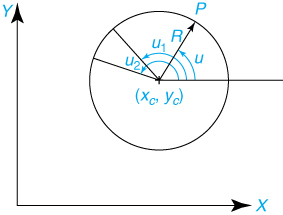
Three angles within a circle. An angle u less than 90 degrees extends as vector R to a point P on the circle. Another angle u 1 is greater than 90 degrees. Another angle u 2 is greater than u 1 but less than 180 degrees. All three angles have the same origin x sub c, y sub c. — **Figure 8.5** Parametric circle

\begin{matrix} P (u) = [\begin{array}{l} x (u) \\ y (u) \end{array}] = [\begin{array}{l} x_{c} + R cos u \\ y_{c} + R sin u \end{array}] 0 \leq u \leq 2 π & (8.11) \end{matrix}

You can normalize the u limits in Eq. (8.11) to (0, 1) instead of (0, 2π). This gives:

\begin{matrix} P (u) = [\begin{array}{l} x (u) \\ y (u) \end{array}] = [\begin{array}{l} x_{c} + R cos 2 π u \\ y_{c} + R sin 2 π u \end{array}] 0 \leq u \leq 1 & (8.12) \end{matrix}

Note that the circle, although closed, has two coincident endpoints, one for each u limit.

The tangent vector of the circle is given by:

\begin{matrix} P' (u) = [\begin{array}{l} x' (u) \\ y' (u) \end{array}] = [\begin{array}{r} - R \sin u \\ R \cos u \end{array}] 0 \leq u \leq 2 π & (8.13) \end{matrix}

Or:

\begin{matrix} P' (u) = [\begin{array}{l} x' (u) \\ y' (u) \end{array}] = [\begin{array}{r} - 2 π R \sin 2 π u \\ 2 π R \cos 2 π u \end{array}] 0 \leq u \leq 1 & (8.14) \end{matrix}

Eq. (8.11) through Eq. (8.14) can also be used to define arcs. The only difference is the u limits (i.e., u₁ ≤ u ≤ u₂). Figure 8.5 shows this arc segment.

Example 8.2

Find the equation of a circle with a radius of 2.0 inches and a center at the origin. Find the midpoint of the circle. What are the tangent vector and slope at this point?

Solution Using Eq. (8.11) with the given data gives:

\begin{matrix} P (u) = [\begin{array}{l} x (u) \\ y (u) \end{array}] = [\begin{array}{l} 2 cos u \\ 2 sin u \end{array}] 0 \leq u \leq 2 π & (8.15) \end{matrix}

The midpoint of the circle occurs in the mid-range of the u parameter (i.e., at u = π). Eq. (8.15) gives:

\begin{matrix} P (π) = [\begin{array}{l} x (π) \\ y (π) \end{array}] = [\begin{array}{r} - 2 \\ 0 \end{array}] & (8.16) \end{matrix}

These coordinates agree with the visual inspection of Figure 8.5; the point is the leftmost point on the circle circumference. Note that the midpoint of the circle is not its center; the center does not lie on the circle circumference. The tangent vector at the midpoint is obtained by substituting u = π in Eq. (8.13) to get:

\begin{matrix} P' (π) = [\begin{array}{l} x' (π) \\ y' (π) \end{array}] = [\begin{array}{r} 0 \\ - 2 \end{array}] & (8.17) \end{matrix}

The slope at this point is given by $\begin{matrix} \frac{y'}{x'} = \infty \end{matrix}$ , as expected, because the tangent vector is vertical at this point; that is, it makes a 90-degree angle measured from the horizontal axis counterclockwise.

8.5 Spline Parametric Equation

Different types of splines exist. The type most commonly used by CAD/CAM systems is the cubic B-spline curve, or spline for short. Figure 8.6 shows a spline connecting n + 1 data points. The spline equation takes the following form:

\begin{matrix} P (u) = f_{0} (u) P_{0} + f_{1} (u) P_{1} + \dots + f_{n} (u) P_{n} u_{\min} \leq u \leq u_{\max} & (8.18) \end{matrix}

A curve u rising from P 0 at u min to P 1 and falls to P and again rises as a curve to P n at u max. A vector extends to P from the origin. — **Figure 8.6** Parametric spline

where the highest degree of any of these f (u) functions is cubic.

Example 8.3

A spline is given by:

\begin{matrix} P (u) = [\begin{array}{l} x (u) \\ y (u) \end{array}] = [\begin{array}{l} 2 + 3 u^{2} - 2 u^{3} \\ 2 + 3 u - 3 u^{2} \end{array}] 0 \leq u \leq 1 & (8.19) \end{matrix}

Find the endpoints and the midpoint of the spline. Also, find the tangent vector and the slope at the midpoint. Using your CAD/CAM system, create the spline defined by Eq. (8.19).

Solution The endpoints occur at u = 0 and u = 1. The midpoint of the spline occurs at u = 0.5. Substituting these values in Eq. (8.19) gives:

P (0) = [\begin{array}{l} 2 \\ 2 \end{array}], P (0.5) = [\begin{array}{l} 2.5 \\ 2.75 \end{array}], a n d P (1) = [\begin{array}{l} 3 \\ 2 \end{array}]

Differentiating Eq. (8.19) gives the tangent vector to the spline at any point on it as:

P' (u) = [\begin{array}{l} 6 u - 6 u^{2} \\ 3 - 6 u \end{array}] 0 \leq u \leq 1

The tangent vector at the midpoint is $P' (0.5) = [\begin{array}{l} 1.5 \\ 0 \end{array}]$ , and the slope is $\frac{y'}{x'} = \frac{0}{1.5} = 0$ ; that is, the tangent vector is horizontal at the midpoint.

The following steps show how to create the spline (see Figure 8.7) using SolidWorks.

Figure 8.7 Spline

Step 1. Create spline: File > New > Part > OK > Front Plane > Spline dropdown on Sketch tab > Equation Driven Curve > Parametric > enter x and y equations and limits given by Eq. (8.19) as shown > ✓ > File > Save As > example8.3 > Save.

8.6 Two-Dimensional Curves

SolidWorks implements the curve parametric theory presented here and provides versatile ways for designers to create curves. Curves may be planar (2D curves) or nonplanar (3D curves). The 2D curves are sketch entities; that is, they lie in the sketch plane, regardless of how complex they may look. To create 2D curves from equations, you can use this sequence (or the sequence shown in Step 1 of Example 8.3): Tools > Sketch Entities > Equation Driven Curve. You must be in a sketch to access it.

8.7 Three-Dimensional Curves

A 3D curve, unlike a 2D curve, does not belong to only one sketch plane. One segment of a 3D curve may belong to one sketch plane, while another segment may belong to another sketch plane. 3D curves are valuable in some designs, and they simplify feature creation significantly, as illustrated in the tutorials in this chapter. 3D curves become more powerful and elegant when you combine them with surfaces, as shown later in the book.

There are multiple ways to create 3D curves, including the following:

Curve explicit equation: This method takes a curve explicit equation in the form given in Eq. (8.1).
Curve parametric equation: This method takes a curve parametric equation in the form given in Eq. (8.3).
3D points: This method requires a list of (x, y, z) coordinates of the 3D points. The user may input the coordinates while creating the curve or store them in a text file and read it into SolidWorks.
3D sketching: This method allows you to sketch entities in different sketch planes.
Composite curve: You can create composite curves by combining curves, sketch geometry, and model edges into a single curve. The individual curves may belong to one sketch or different sketches. If they belong to the same sketch, the resulting composite curve is 2D. If they belong to multiple sketches, the resulting curve is 3D.
Curve projected onto a model face: You can convert a 2D curve created on a sketch plane into a 3D curve by projecting it onto a model face. The model face needs to be nonplanar to create a 3D curve; otherwise, the projected curve remains 2D.
Projected curve: This is a very powerful method to create 3D curves. You can create a 3D curve from two 2D curves. These 2D curves are two projections of the 3D curve onto two intersecting sketch planes. The 3D curve represents the intersection of the two extruded surfaces generated by two 2D curves, as shown in Figure 8.8. A common practice is to sketch the two best projections of the 3D curve on two different sketches (e.g., front and top or front and right) and then use the projected curve method to create the 3D curve. If the resulting curve needs to be tweaked, you can delete it, modify the two sketches, and then re-create it. You continue this iterative process until you are satisfied with the resulting 3D curve.

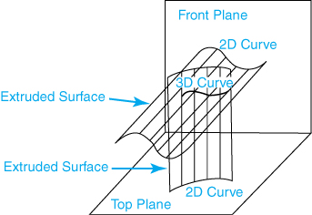
An illustration of a 90-degree front and top plane with a horizontal extruded surface on top of a vertical extruded surface placed on the top plane. The curve at the intersection of two surfaces is labeled 3 D curve. — **Figure 8.8** Creating a 3D projected curve

The chapter tutorials illustrate how to use these methods.

8.8 Curve Management

After you create curves, you can manage and manipulate them in different ways. You can modify, edit, trim, split (divide), and/or intersect them. These manipulations are easily done as an outcome of the curve parametric formulation presented in this chapter. You have already done all these manipulations except breaking a curve. Follow this sequence to split a curve: Right-click it > Split Entities (from the popup window) > click the curve where you want to split it > Esc key on the keyboard to finish. To verify the split, hover over the entities and observe the curve segments. You can also verify the split by right-clicking a segment > Delete from the popup menu.

8.9 Tutorials

The tutorials in this chapter allow you to practice creating and using curves. The tutorials show how to use all the methods for creating 3D curves covered so far.

Tutorial 8–1 Create a 2D Curve by Using an Explicit Equation

You create a curve defined by using the following explicit equation:

\begin{matrix} y = 0.5 x^{2} 0 \leq x \leq 3 & (8.20) \end{matrix}

Eq. (8.20) defines half a parabola that is symmetric with respect to the Y axis. You revolve the parabola to create a feature for better visualization (see Figure 8.9).

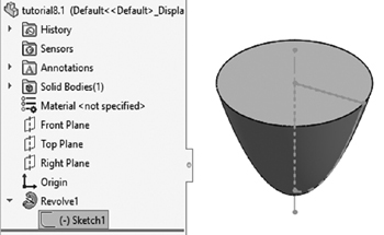
An illustration of a parabola with the axis of symmetry highlighted. A menu on the left shows the sketch 1 option under the Revolve 1 drop-down menu. — **Figure 8.9** A revolve

Step 1: Create Sketch1 and Revolve1-Paraboloid: File > New > Part > OK > Front Plane > Spline dropdown on Sketch tab > Equation Driven Curve > Explicit > enter equation and limits given by Eq. (8.20) as shown > ✓ > Line on Sketch tab > sketch horizontal and vertical lines shown to close cross section > Centerline on Sketch tab > sketch vertical line shown passing through origin > exit sketch > Revolved Boss/Base on Features tab > ✓ > File > Save As > tutorial8.1 > Save.

An illustration of a parabola with the axis of symmetry and the section of the parabola highlighted. A menu displays the Explicit radio button selected and the parameters displaying the equation y x, x 1, and x 2.

Tutorial 8–2 Create a 2D Curve by Using a Parametric Equation

You can create a curve defined by the following parametric equation:

\begin{matrix} P (u) = [\begin{array}{l} x (u) \\ y (u) \end{array}] = [\begin{array}{l} 3 u^{3} - 2 u^{2} + u \\ 5 u + 1 \end{array}] 0 \leq u \leq 1 & (8.21) \end{matrix}

You can revolve the resulting curve to create a feature (see Figure 8.10) for better visualization.

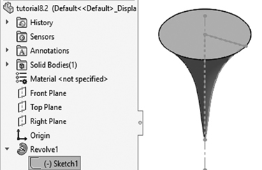
An illustration of a top with a sharp vertex with the axis of symmetry highlighted. A menu on the left shows the sketch 1 option under the Revolve 1 drop-down menu. — **Figure 8.10** A revolve

Step 1: Create Sketch1 and Revolve1: File > New > Part > OK > Front Plane > Spline dropdown on Sketch tab > Equation Driven Curve > Parametric > enter equation and limits given by Eq. (8.21) as shown > ✓ > Line on Sketch tab > sketch horizontal and vertical lines shown to close cross section > Centerline on Sketch tab > sketch vertical line shown passing through origin > exit sketch > Revolved Boss/Base on Features tab > ✓ > File > Save As > tutorial8.2 > Save.

An illustration of a top with a sharp vertex and a section of the parabola highlighted. A menu displays the Parametric radio button selected and the parameters displaying the equation x t, y t, t 1, and t 2.

Tutorial 8–3 Create a 3D Curve by Using a Parametric Equation

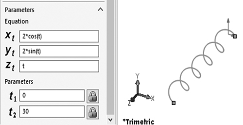
You can create a helix defined by the following parametric equation:

\begin{matrix} P (u) = [\begin{array}{l} x (u) \\ y (u) \\ z (u) \end{array}] = [\begin{array}{l} 2 cos u \\ 2 \sin \\ u \end{array}] 0 \leq u \leq 30 & (8.22) \end{matrix}

You can sweep a circle along the resulting helix to create a feature for better visualization (see Figure 8.11).

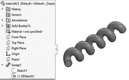
An illustration of a section of spring with thick spirals. A menu on the left shows the sketch 1 options under the Sweep 1 drop-down menu. — **Figure 8.11** A sweep

Step 1: Create 3D curve: File > New > Part > OK > Sketch dropdown on Sketch tab > 3D Sketch > Spline dropdown on Sketch tab > Equation Driven Curve > enter equation and limits given by Eq. (8.22) as shown > ✓ > File > Save As > tutorial8.3 > Save.

An illustration of spring with two ends. A menu displays the equation x t, y t, z t, t 1, and t 2.

Step 2: Create plane perpendicular to curve endpoint: Reference Geometry dropdown on Features tab > Plane > helix endpoint shown > ✓.

An illustration of a plane with one end of the spring attached at the center. A menu displays message, first reference, and second reference drop-down menus.

Step 3: Create sweep: Select Plane1 created in Step 2 as sketch plane > Circle on Sketch tab > click helix endpoint and drag to sketch a circle with diameter of 3.0 inches > exit sketch > Swept Boss/Base > circle sketch as profile and helix sketch as path as shown > ✓.

Note: You use a 3D sketch in Step 1 to have access to the z coordinate of the parametric equation, as shown. If you use a 2D sketch as in Tutorial 8–2, the z coordinate does not appear.

Tutorial 8–4 Create a 3D Curve by Using 3D Points

Here you create a set of 3D points in 3D modeling space and connect them with a spline. You can use the resulting curve to create a sweep for better visualization (see Figure 8.12). All dimensions in this tutorial are in millimeters.

A model of a rod bent in the form of a circle with extending ends. A menu on the left shows the sketch 1 options under the Sweep 1 drop-down menu. — **Figure 8.12** A sweep

Step 1: Create 3D curve, Curve1, by entering 3D points: File > New > Part > Insert > Curve > Curve Through XYZ Points > double-click any cell to enter value > enter all values shown > OK.

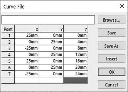
A curve file window showing the browse button with a search bar and a table below displaying the 7 measurement points for x, y, and z. The Ok button is selected.

Note: You can save the points’ coordinates in a text file and read them in instead of typing as follows: Browse button shown > locate the file > Open > OK. The file format is as follows: one line per point. Point coordinates (x, y, z) are separated by spaces, as follows:

25 0 16
0 25 4
–25 0 8

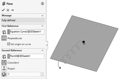
Step 2: Create plane perpendicular to curve endpoint: Reference Geometry dropdown on Features tab > Plane > select curve as First Reference > select curve endpoint shown as Second Reference > ✓.

An illustration of a plane with one end of the curved string attached at the center and the other end is free. A menu displays message, first reference, and second reference drop-down menus.

Step 3: Create Sketch1: Select plane created in Step 2 as a sketch plane > Circle on Sketch tab > click curve end and drag and sketch and dimension circle as shown > exit sketch.

An illustration of a circle with a line measuring 5.00 passing through the center cutting it in half.

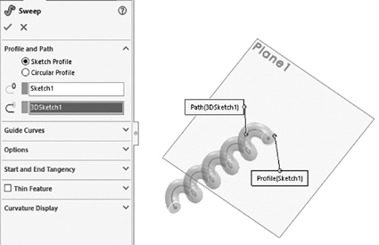
Step 4: Create sweep for better visualization: Swept Boss/Base on Features tab > Sketch1 as profile > Curve1 as path > ✓ > File > Save As > tutorial8.4 > Save.

Tutorial 8–5 Create a 3D Curve by Using 3D Sketching

Here you build a bicycle handlebar using a 3D sketch. Enable sketching in 3D space by toggling (changing) sketch planes. You toggle by using the Tab key on the keyboard. The available sketch planes are XY (front), XZ (top), and YZ (right). The current plane designation is attached to the mouse as it moves. The bicycle handlebar requires the XY plane and the YZ plane. Figure 8.13 shows the handlebar. All dimensions in this tutorial are in inches.

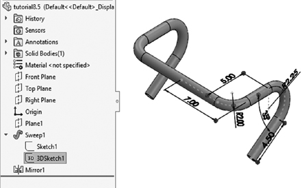
An illustration of a horizontal rod with perpendicularly downward bent at 35 degrees on both ends. One half of the rod measures 7.00 till the bend and the perpendicular bend measures 5.00. The downward extending end measures 4.50. A menu on the left shows the 3 D sketch 1 option selected from the Sweep 1 drop-down menu. — **Figure 8.13** Bicycle handlebar

Step 1: Create 3DSketch1: File > New > Part > OK > Sketch dropdown on Sketch tab > 3D Sketch > Line on Sketch tab > click origin and drag along the X-axis to sketch a line in the XY plane as shown > Tab key twice to switch to ZX plane > Line on Sketch tab > sketch line > Arc dropdown on Sketch tab > Tangent Arc > sketch (in YZ plane) an arc passing through endpoint of line as shown > Line on Sketch tab > sketch (in YZ plane) a line passing through endpoint of arc as shown > Esc > line + Ctrl key + arc > Tangent from Add Relations box > ✓ > fillet two lines as shown > Smart Dimensions on Sketch tab > dimension all as shown > Save As > tutorial8.5 > Save.

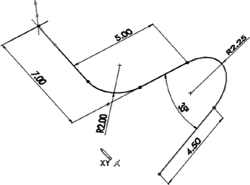
An illustration of a line that bends to a spline of 35 degrees. The line with the bend measures 7.00. The rising side of the spline from the line measures 5.00. The falling end of the spline measures 4.50.

Step 2: Fully define 3DSketch1: Centerline on Sketch tab > sketch line connecting the arc center and line endpoint as shown> right-click > select Make Along Y relation from menu shown > exit sketch.

An illustration of a spline of 35 degrees and R 2.25. A menu on the left displays the existing relations, add relations, and options drop-down menus. The check box, For construction, is selected under options.

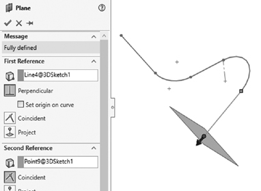
Step 3: Create a Plane1: Reference Geometry dropdown on Features tab > Plane > Perpendicular > line segment shown > line endpoint shown > ✓.

An illustration of a spline curve from a straight line. The spline end is attached to a plane with an arrow pointing on the other side of the plane. A menu on the left displays the message, first reference, and second reference drop-down menus.

Step 4: Create Sketch1: Select Plane1 created in Step 3 as a sketch plane > Circle on Sketch tab > click line end and drag and sketch and dimension circles as shown > exit sketch.

An illustration of a circle with an inner circle as a lining. The outer circle diameter measures 1.00 and the inner circle measures 0.90.

Step 5: Create Sweep1 for better visualization of curve: Swept Boss/Base on Features tab > Sketch1 as profile > 3DSketch3 as path > ✓.

Step 6: Create other half of bike handlebar: Mirror on Features tab > expand feature tree > Right Plane as Mirror Face/Plane as shown > Sweep1 as Features to Mirror, as shown > ✓.

An illustration of plane 1 with one end of a transparent spline tube with lining inside is attached at the center and the other end passes through an outline labeled right plane. A menu displays the Mirror face or plane, features to mirror, faces to mirror drop-down menus. Another list with the right plane and sweep 1 from plane 1 selected.

Tutorial 8–6 Create a 3D Curve by Using Composite Curves

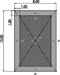
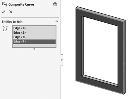
Here you create a picture frame by using a composite curve consisting of all the outside edges of the frame. You use the composite curve to create a sweep to model the decorative routing of the frame, as shown in Figure 8.14. All dimensions in this tutorial are in inches.

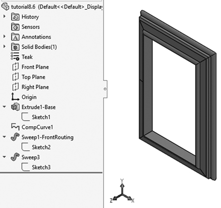
An illustration of a photo frame with a thick three-layered frame. A menu on the left shows the sketch 1, 2, and 3 options from the Extrude 1 Base, Sweep 1 front routing and Sweep 3 dropdowns respectively. — **Figure 8.14** Picture frame with decorative routing

Step 1: Create Sketch1 and Extrude1-Base feature: File > New > Part > Front Plane > Extruded Boss/Base on Features tab > Center Rectangle on Sketch tab > sketch and dimension two center rectangles shown > exit sketch > enter 0.5 for D1 > reverse extrusion direction > ✓ > File > Save As > tutorial8.6 > Save.

An illustration of a rectangle of width 8.00 and height 12.00 with an inner rectangle. The distance between both measures 1.00.

Step 2: Create CompCurve1: Insert menu > Curve > Composite > select the four edges of the outer rectangle created in Step 1 in counterclockwise direction > ✓.

An illustration of a rectangular photo frame with a composite curve menu on the left displaying entities to join drop down with edge 4 option selected.

Step 3: Create Sketch2 and Sweep1-FrontRouting feature: Top Plane > Line on Sketch tab > sketch and dimension lines shown > Arc dropdown on Sketch tab > 3 Point Arc from dropdown > sketch and dimension arc shown > exit sketch > Swept Boss/Base on Features tab > Sketch2 for profile and CompCurve1 for path > ✓.

An illustration of a rectangle with an indefinite shape attached to it at the bottom of length 1.00, falling from 45 degrees to 10 degrees and a spline of R 0.25. The width of the shape is 0.50.

Step 4: Create Sketch3: Top Plane > Circle on Sketch tab > sketch and dimension circle shown (make sure to snap to intersection point as shown) > exit sketch.

An illustration of a circle and a rectangle. The circle is cut half by a line at 0.50. The left-up corner of the rectangle is at the center of the circle.

Step 5: Create Sweep2-BackRouting feature: Swept Boss/Base on Features tab > Sketch3 for profile and CompCurve1 for path > ✓.

Step 6: Change material to teak wood: Right-click Material node > Edit Material > Woods > Teak > Apply > Close.

Tutorial 8–7 Create a 3D Curve by Projecting a Sketch onto a Curved Face

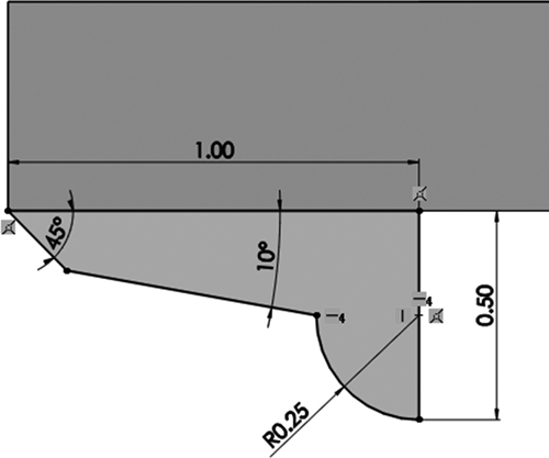
Here you use a curve projected onto a cylindrical face to engrave a part, as shown in Figure 8.15. All dimensions in this tutorial are in inches.

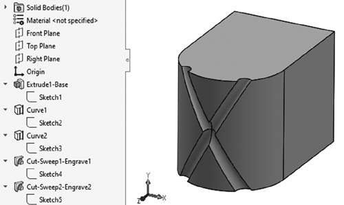
An illustration of a square block with one curved side. The curved side is engraved with a big X. A menu on the left shows the sketch 1, 2, 3, 4, and 5 options from the Curve and Cut sweep drop-down menus. — **Figure 8.15** Engraving the letter X on a curved face

Step 1: Create Sketch1 and Extrude1-Base feature: File > New > Part > Top Plane > Extruded Boss/Base on Features tab > Line on Sketch tab > sketch and dimension lines shown > Arc dropdown on Sketch tab > 3 Point Arc > sketch and constrain arc shown > exit sketch > enter 4.0 for D1 > reverse extrusion direction > ✓ > File > Save As > tutorial8.7 > Save.

Three illustrations. The first sketch shows the square with one curved side. The square sides measure 4.00. The second illustration show s a sketch of a square with a diagonal line from the top left off-center of 1.20 from the center. The third illustration shows a square block with one curved side. The curved side has a diagonal line. A projected curve menu shows the sketch on faces projection selected.

Step 2: Create Sketch2 and Curve2: Front Plane > Line on Sketch tab > sketch and dimension line shown above > exit sketch > Insert Curve > Projected > select Sketch On Faces for Projection Type > expand feature tree > Sketch2 and curved face as shown > ✓. Repeat Step 2 for other portion of X shape.

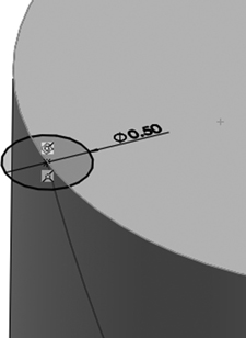
Step 3: Create Sketch3: Top Plane > Point on Sketch tab > click somewhere near top face of Extrude1-Base feature > Esc key > select point just created + Ctrl key + Curve2 > Pierce in Add Relations section > ✓ > Circle on Sketch tab > click point and drag to sketch and dimension circle with a 0.5 inch diameter > exit sketch. Repeat Step 3 for other portion of X shape.

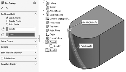
An illustration of the curved edge of a curved block. The tip is circled and labeled 0.50 angle

Step 4: Create Cut-Sweep1-Engraved1 feature: Swept Cut on Features tab > Sketch3 for profile and Curve1 for path > ✓. Repeat Step 4 for other portion of X shape.

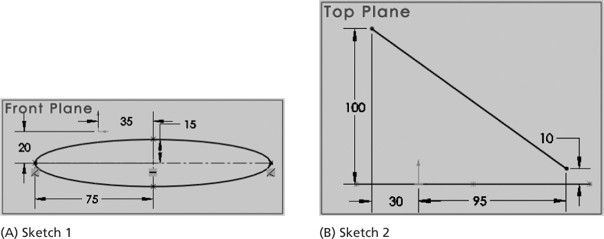
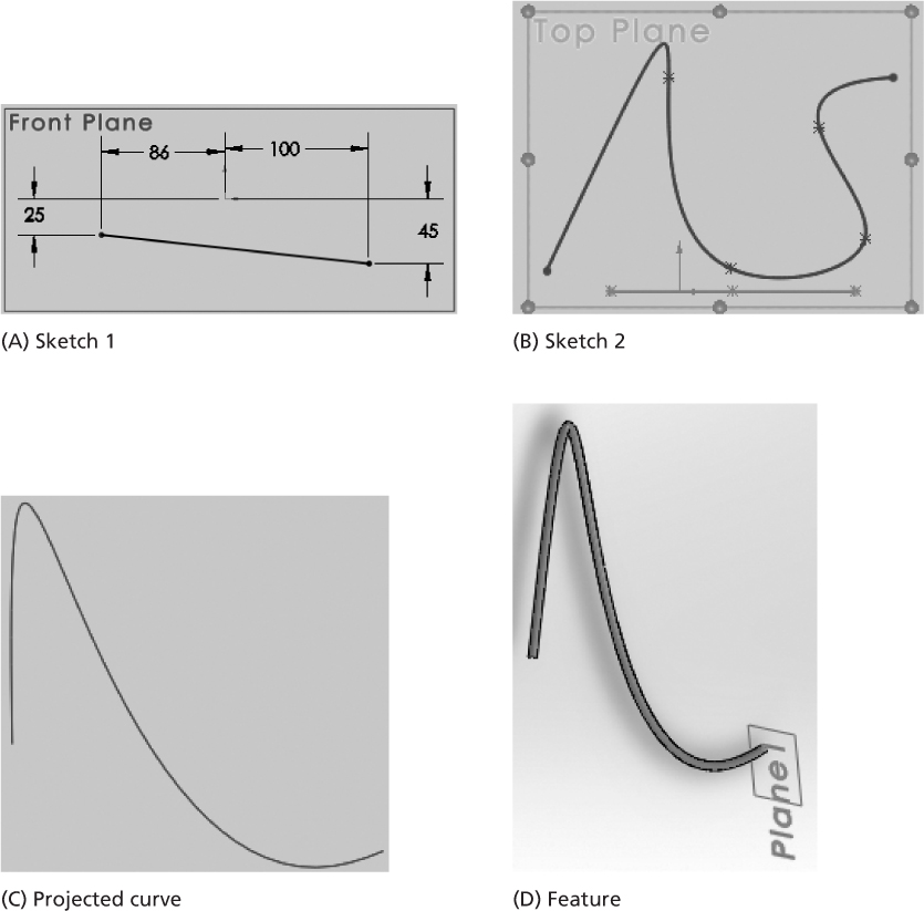
Tutorial 8–8 Create a 3D Curve Using Projected Curves

Here you create a 3D curve from projected curves (2D sketches). By projecting two 2D curves from multiple sketch planes, you can create a 3D curve. This tutorial shows examples of creating various solids using different projected sketches and a sweep profile. Case 1 (see Figure 8.16) is shown in detail. The remaining cases are illustrated but are not shown in detail; the Case 1 steps can be followed in order to create the other cases. You create 3D curves using the following 2D curves:

An illustration of Plane 1 with a cylinder at the center perpendicular to it. A menu on the left shows Curve 1 drop-down menu with sketch 1 and 2 options. — **Figure 8.16** Case 1: Two lines

Case 1: Use two lines.

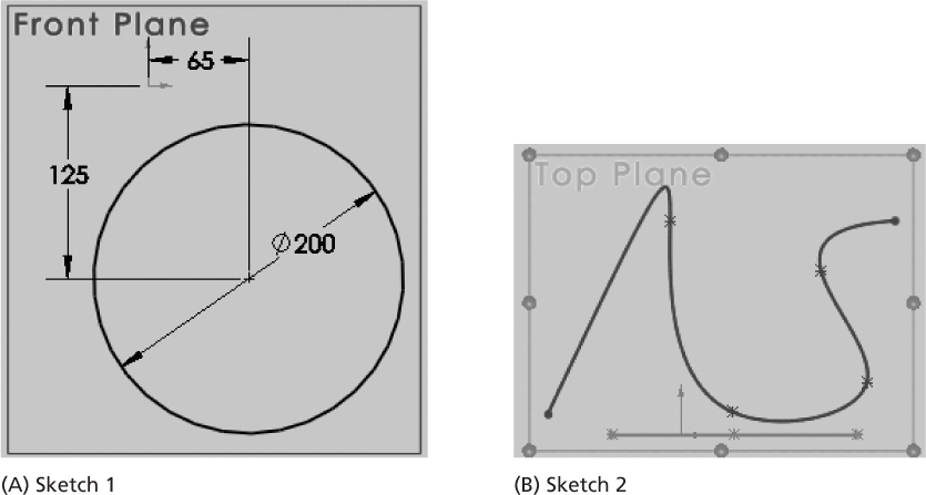
Case 2: Use two circles.

Case 3: Use two arcs.

Case 4: Use a line and a circle.

Case 5: Use a line and an arc.

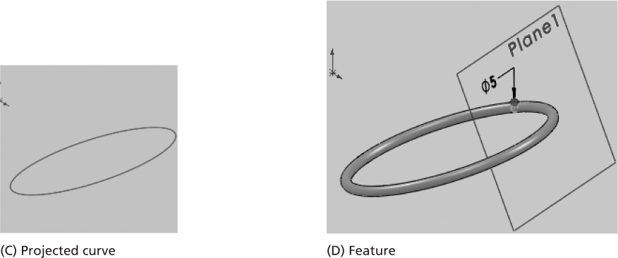
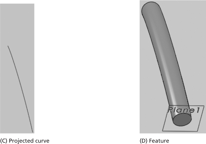
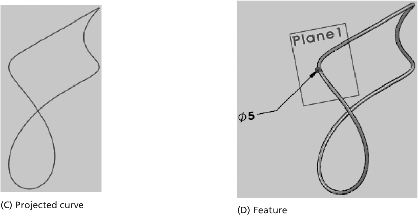
Case 6: Use two ellipses.

Case 7: Use an ellipse and a line.

Case 8: Use an ellipse and a circle.

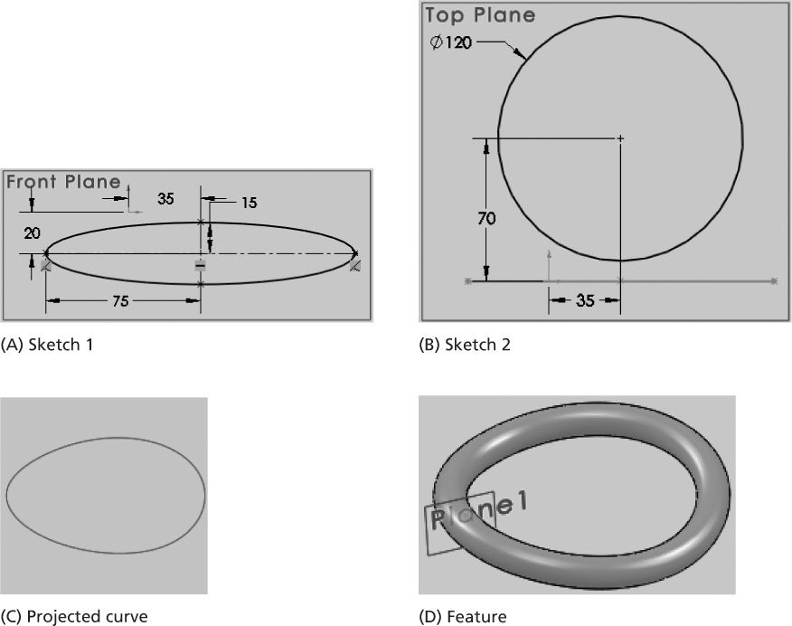
Case 9: Use an ellipse and an arc.

Case 10: Use two splines.

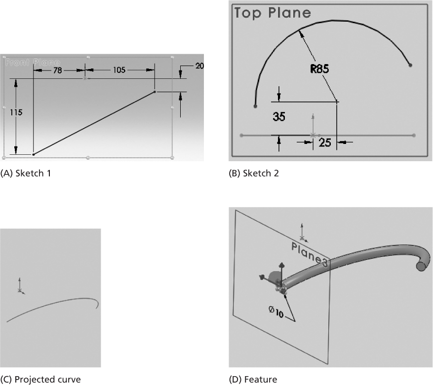
Case 11: Use a spline and a line.

Case 12: Use a spline and a circle.

Case 13: Use a spline and an ellipse.

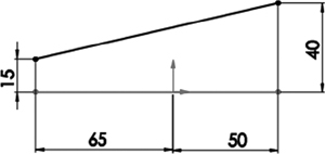
Step 1: Sketch Sketch1: File > New > Part > Tools > Options > Document Properties tab > Units > MMGS > OK > Front Plane > Line on Sketch tab > sketch and dimension line shown > exit sketch > File > Save As > tutorial8.8 > Save.

An illustration of a sloping line measuring 65 and 50. The height of the line measuring 56 is 40.

Step 2: Create Sketch2: Repeat Step 1 to create the sketch shown. Use Top Plane to create the sketch.

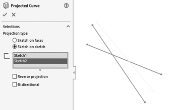
An illustration of a rising line and a horizontal line in parallel measuring 65 and 50. The space between the two lines is 15 on the starting and 40 on the end.

Step 3: Create projected curve: Insert > Curve > Projected > expand feature tree > Sketch1 > Sketch2 > ✓.

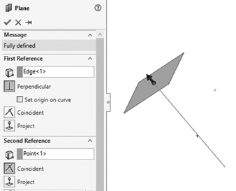
An illustration of two intersecting lines. A Projected Curve menu on the left shows the sketch on the sketch radio button selected.

Step 4: Create Plane1: Reference Geometry on Features tab > Plane > Curve1 > Perpendicular > endpoint shown > ✓.

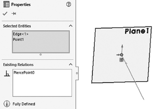
An illustration of a line passing through the center of a plane. A plane menu shows the message, first reference, and second reference drop-down menus.

Step 5: Create Sketch3: Select Plane1 as sketch plane > Point on Sketch tab > sketch point shown > Esc key > point just created + Ctrl key + Curve1 > Pierce from Add Relations section > ✓ > Circle on Sketch tab > click point and drag to sketch and dimension circle with 25 mm diameter > exit sketch.

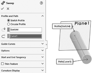
An illustration of plane 1 with a line passing at the center. A properties pane on the left shows the selection entities and existing relations drop-down menus.

Step 6: Create Sweep1: Swept Boss/Base on Features tab > Sketch3 for profile and Curve1 for path > ✓.

Case 2: Two circles

Case 3: Two arcs

A case of a line and a circle is presented.

Case 4: A line and a circle

A case of a line and an arc is presented.

Case 5: A line and an arc

Case 6: Two ellipses

A case of an ellipse and a line is presented.

A figure shows the projected curve and a feature.

Case 7: An ellipse and a line

A case of an ellipse and a circle is presented.

Case 8: An ellipse and a circle

A case of an ellipse and an arc is presented.

Case 9: An ellipse and an arc

Case 10: Two splines

A case of a spline and a line is presented.

Case 11: A spline and a line

A case of a spline and a circle is presented.

Case 12: A spline and a circle

A case of a spline and an ellipse is presented.

Case 13: A spline and an ellipse

Tutorial 8–9 Create a Stethoscope Model

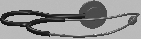
Here you use 2D and 3D (projected) curves to create the stethoscope model shown in Figure 8.17. All dimensions in this tutorial are in inches.

An illustration of a stethoscope. A menu on the left shows drop-down menus with sketch 1 to sketch 9 options. — **Figure 8.17** A stethoscope

Step 1: Create Sketch1: File > New > Part > Top Plane > Spline on Sketch tab > starting at origin, sketch spline shown > exit sketch > File > Save As > tutorial8.9 > Save.

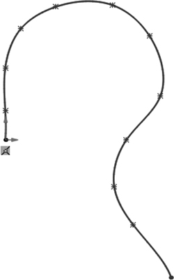
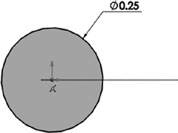
An illustration of a curved line with an arch shape and the right end of the arch bends inward into a curve.

Step 2: Create Sketch2 and Sweep1-RubberTube: Front Plane > Circle on Sketch tab > sketch and dimension circle shown > exit sketch > Swept Boss/Base on Features tab > Sketch2 as profile > Sketch1 as path > ✓.

An illustration of a circle measuring 0.25 with a horizontal line extending out to the right from the center.

Step 3: Create Sketch3: Top Plane > Arc dropdown on Sketch tab > 3 Point Arc > sketch and dimension half circle shown > exit sketch.

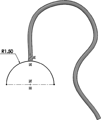
An illustration of the stethoscope's tube from the top of a semi-circle. The semi-circle is labeled R 1.50.

Step 4: Create Plane1: Reference Geometry dropdown on Features tab > Plane > arc created in Step 3 > Perpendicular > arc endpoint shown > ✓.

An illustration of a plane with the one end of a semi-circle at the center of the plane perpendicularly. A plane menu on the left shows the message, first reference, and second reference drop-down menus.

Step 5: Create Sketch4 and Sweep2-DoubleTube: Select Plane1 as a sketch plane > Circle on Sketch tab > click endpoint of arc shown > Esc key > circle just created + Ctrl key + circle of Sketch2 > Equal from Add Relations section > ✓ > Swept Boss/Base on Features tab > Sketch4 as profile > Sketch3 as path > ✓.

An illustration of plane 1 with the one end of a semi-circle at the center of the plane perpendicularly.

Step 6: Fillet the tubing: Fillet on Features tab > hover over intersection area and select as shown > use 0.5 in. for fillet radius > ✓.

An illustration of an intersection of two tubular structures. The intersection is labeled Radius 0.5 inches.

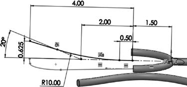
Step 7: Create Sketch5: Top Plane > Line on Sketch tab > sketch lines shown > Arc dropdown on Sketch tab > 3 Point Arc > sketch arc shown > dimension as shown > exit sketch.

An illustration of an arch-shaped tube with one end extending as a curved line at 10 degrees of height 3.00 as a straight line, 0.90 as a curved line, and the curve is labeled R 1.00.

Step 8: Create Sketch6: Right Plane > Line on Sketch tab > sketch and dimension two lines shown > Arc dropdown on Sketch tab > 3 Point Arc > sketch and dimension arc shown > exit sketch.

An illustration of a horizontal line of length 4.00 and moves up and down at an angle 20 degrees from the length 2.00. The height of the movement is 0.625. The line extends to the stethoscope tube on the right. The Upward lifted line is labeled R 10.00.

Step 9: Create Curve1: Insert > Curve > Projected > Sketch5 > Sketch6 > ✓.

An illustration of a curved line from the stethoscope's arch-shaped tube's center. A projected curve menu on the left shows the sketch on the sketch radio button selected under projection type and sketch 6 is selected.

Step 10: Create Sketch7 and Sweep3-MetalTubing: Face shown of Sweep2-DoubleTube > Circle on Sketch tab > sketch concentric circle and dimension as shown > exit sketch > Swept Boss/Base on Features tab > Sketch7 for profile and Curve1 as path > ✓.

An illustration of a circle with a shaded circle inside of angle 0.15.

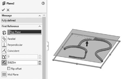
Step 11: Create Plane 2: Reference Geometry dropdown on Features tab > Plane > expand feature tree > Top Plane > enter 0.625 for D1 > ✓.

An illustration of a stethoscope placed on a top plane. A plane 2 menu on the left shows the message and the first reference drop-down with Top plane selected.

Step 12: Create Sketch8: Select Plane2 as sketch plane > Line on Sketch tab > sketch and dimension lines shown > Sketch Fillet on Sketch tab > fillet and dimension corners shown > Line on Sketch tab > Centerline > sketch horizontal line shown > exit sketch.

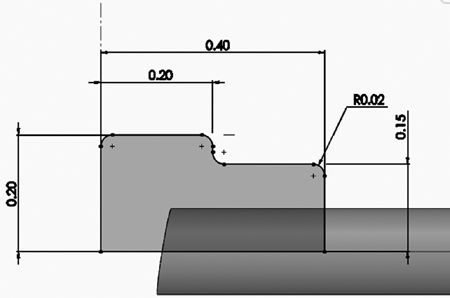
A sketch of a rectangle of width 0.40 and the top side of the rectangle slopes down from 0.20. The height of the rectangle is 0.20 and the height is reduced to 0.15 after the slope. The top side has curved corners of R 0.02.

Note: The vertical construction line begins at the model origin.

Step 13: Create Revolve1-Earplug: Select Sketch8 > Revolved Boss/Base on Features tab > bottom edge line of Sketch8 as Axis of Revolution > ✓.

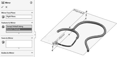
Step 14: Create other half: Mirror on Features tab > expand feature tree > Right Plane as Mirror Face/Plane > Sweep3-MetalTubing > Revolve1-Earplug > ✓.

An illustration of a stethoscope placed on plane 2. Another perpendicular front plane passes at the center. A mirror menu on the left shows the mirror face or plane dropdown with the right plane selected and the features to mirror drop down with revolve 1 earplug option selected.

Step 15: Create Sketch9 and Revolve2-DiaphragmHousing: Top Plane > Revolved Boss/Base on Features tab > Line on Sketch tab > sketch and dimension lines shown > exit sketch > line touching Sweep2-DoubleTube as Axis of Revolution > ✓.

An illustration of a plane with a cut in the center making it have a left and right leg. The left leg is 0.50 and the right leg is 0.75. The width of the plane is 0.50 and the width of the cut is 0.25. The height of the plane without the cut is 0.25. A vertical rod extends above on top of the plane.

Problems

1 What is the difference between analytic and synthetic curves? Which family is better? Why?

2 If a parametric curve has u limits of u_min and u_max, what is the u value at its midpoint?

3 Use the tangent vector Eq. (8.4) to find the curve slopes in the XY, XZ, and YZ planes.

4 Find the parametric equation of the line connecting point (2, 1, 0) to point (–2, –5, 0). Find the line midpoint and its tangent vector. Sketch the line and show the endpoints and the parameterization direction on the sketch.

5 For the line in Problem 4, find the coordinates of the points located at u = 0.25 from both ends of the line.

6 Reverse the parameterization direction of the line in Problem 4 and solve the problem again.

7 Repeat Problems 4 and 5 but for points (1, 3, 7) and (–2, –4, –6).

8 Find the slopes of the lines in Problem 7 in the XY, XZ, and YZ planes.

9 Find the equation of a circle with a diameter of 3.0 inches and a center at (1, –2). Find the four quarter points on the circle. Use Eq. (8.12). What are the tangent vectors and slopes at these points?

10 Repeat Problem 9 but for a circle with a radius of 1 inch and a center at the origin.

11 Use both Eqs. (8.11) and (8.12) to write the equation of an arc whose diameter is 1.5 inches and that is located in the third quadrant with a center at the origin.

12 A spline is given by:

P (u) = [\begin{array}{l} x (u) \\ y (u) \end{array}] = [\begin{array}{l} 1 + 4 u - u^{2} \\ 2 - u + u^{2} \end{array}] 0 \leq u \leq 1

Find the endpoints and the midpoint of the spline. Also, find the tangent vector and the slope at the midpoint. Using your CAD/CAM system, create the spline defined by this equation.

13 A spline is given by:

P (u) = [\begin{array}{l} x (u) \\ y (u) \end{array}] = [\begin{array}{l} - 2 - 2 u^{2} \\ - 1 + u - 2 u^{2} \end{array}] 0 \leq u \leq 1

Find the endpoints and the midpoint of the spline. Also, find the tangent vector and the slope at the midpoint. Using your CAD/CAM system, create the spline defined by this equation.

14 A spline is given by:

P (u) = [\begin{array}{l} x (u) \\ y (u) \end{array}] = [\begin{array}{l} 2 u \\ 2 - u \end{array}] 0 \leq u \leq 1

What shape is this spline? Why? Verify your answer by creating it on your CAD/CAM system.

15 Use your CAD/CAM system to create a revolve defined by the following explicit equation of an ellipse:

\frac{x^{2}}{{(6.5)}^{2}} + \frac{y^{2}}{{(3)}^{2}} = 1 - 6.5 \leq x \leq 6.5

16 Use your CAD/CAM system to create a revolve defined by the following parametric equation of a spline:

\begin{array}{l} x (u) = 3 u^{2} - 2 u + 2 0 \leq u \leq 1 \\ y (u) = - 3 u^{2} + 3 u + 2 0 \leq u \leq 1 \end{array}

17 Table 8.1 shows the (x, y, z) coordinates of 3D points that define the two edges (profiles) of a laboratory chair. Create each edge. Sweep a circle with radius of 1/2 inch along each curve. All dimensions are in inches.

Table 8.1 3D Points of the Edges of a Laboratory Chair

(A) Curve for Edge 1

-7		0
	1	0.5
-7	2	0.5
-7	5	0
-7	9	1
-5.5	9	3
-5.5	8.5	5
-5.5	9	10

(B) Curve for Edge 2

7	0	0
7	1	0.5
7	2	0.5
7	5	0
7	9	1
5.5	9	3
5.5	8.5	5
5.5	9	10

18 Figure 8.18 shows the front and top sketches of half the profile of a skateboard. Use your CAD/CAM system to create the 3D curve that represents the skateboard profile. Sweep a circle with a radius of 1/2 inch along the curve. All dimensions are in inches.

The 2D projections of a skateboard profile are shown. The front plane sketch shows the half profile of the skateboard. The profile is symmetric about the vertical axis. A horizontal line of length 6.00 inches is drawn from the vertical axis. Then, the profile follows a curved path in the upward direction. The endpoint of the curve is at a height 2 inches from the horizontal line. The total length of half the profile of the skateboard is 11.00 inches. The top plane sketch is symmetric about the vertical axis. It shows a horizontal line of length 6.00 inches from the vertical axis. Then, the profile follows a curved path. Here, the curved path is created using the spline feature. The midpoint of the spline is at a distance of 9.00 inches from the vertical axis. The midpoint of the skateboard profile is at a distance of 4.00 inches from the profile edges.

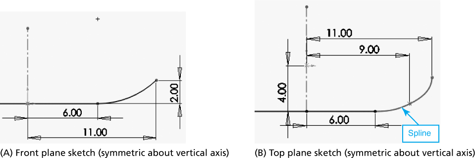
Figure 8.18 2D projections of a skateboard profile

19 Figure 8.19 shows the front and right sketches of a bicycle helmet. Use your CAD/CAM system to create the 3D curve that represents the helmet profile. Sweep a circle with a radius of 1/2 inch along the curve. All dimensions are in inches.

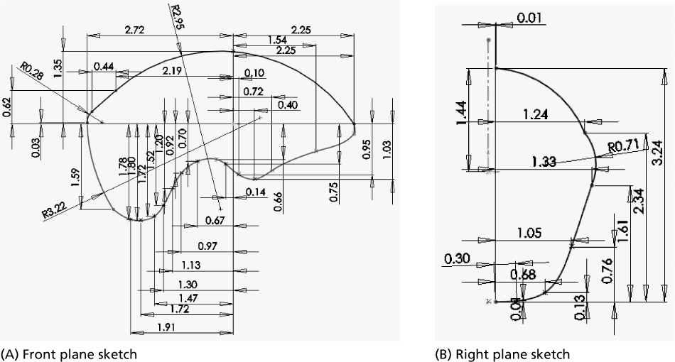
A figure shows the front plane and right plane sketches of a bicycle helmet. — **Figure 8.19** 2D projections of a bicycle helmet profile

20 Figure 8.20 shows the front and right sketches of the profile of a weed whacker debris shield. Use your CAD/CAM system to create the 3D curve that represents the profile. Sweep a circle with a radius of 1/2 inch along the curve. All dimensions are in inches.

Figure 8.20 2D projections of the profile of a weed whacker debris shield

21 Figure 8.21 shows the front and left sketches of the profile of an S-shaped chair. Use your CAD/CAM system to create the 3D curve that represents the profile. Sweep a circle with a radius of 1/2 inch along the curve. All dimensions are in millimeters.

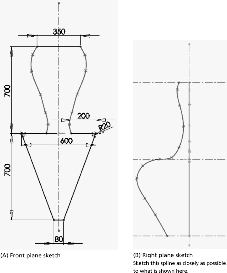
A figure depicts the front plane sketch and the right sketch of an S-shaped chair. — **Figure 8.21** 2D projections of the profile of an S-shaped chair

22 Figure 8.22 shows the top and front sketches of the profile of a bike seat. Use your CAD/CAM system to create the 3D curve that represents the profile. Sweep a circle with a radius of 1/2 inch along the curve. All dimensions are in inches.

In the top plane sketch, the profile is symmetric about the horizontal axis. The profile of the fuel tank is wider compared to the seat portion. A slot exists at the center of the fuel tank profile. It represents the fuel input region. The distance between the curved profile of the fuel tank and the horizontal reference line is 2.70 units. A series of points are marked on the profile from the tank region to the tail of the seat region. The vertical dimensions of these points from the horizontal reference axis are 0.40, 0.85, 1.15, 2.20, and 2.70 units. The total length of the profile is 10.52 units. The horizontal distances of the profile points from the tail section of the seat are 1.66, 5.50, 8.50, and 10.03 units. In the front plane sketch, the profile is represented by a curve. It shows a horizontal line followed by a slope. The dimensions on the left section are 1.33, 1.66, 2.11, 2.19, and 2.21 units. A series of points are marked on the profile. The orientation triad is present at the center of the seat profile. The horizontal distances of the points present to the left of the vertical reference axis are 0.23, 3.52, 5.33, 6.11. and 6.51 units. The horizontal distances of the points present in the tail section are 3.75, 4.09, and 5.06 units.

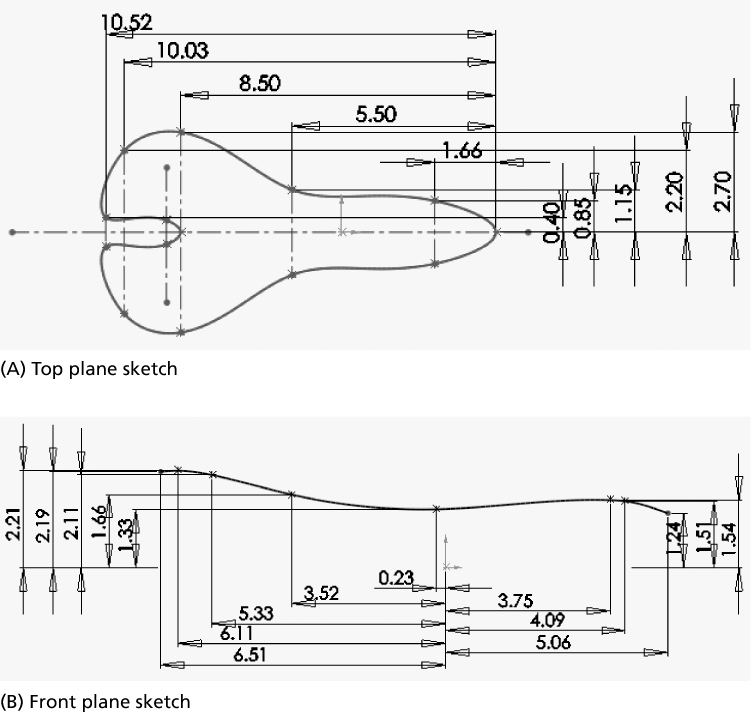
Figure 8.22 2D projections of the profile of a bike seat

..................Content has been hidden....................

You can't read the all page of ebook, please click here login for view all page.