
In the preceding section, we had a brief discussion of what is referred to as descriptive statistics. In this section, we will discuss what is known as inferential statistics whereby we try to use characteristics of the sample dataset to draw conclusions about the wider population as a whole.
One of the most important methods in inferential statistics is hypothesis testing. In hypothesis testing, we try to determine whether a certain hypothesis or research question is true to a certain degree. One example of a hypothesis would be this: Eating spinach improves long-term memory.
In order to investigate this question by using hypothesis testing, we can select a group of people as subjects for our study and divide them into two groups or samples. The first group will be the experimental group, and it will eat spinach over a predefined period of time. The second group, which does not receive spinach, will be the control group. Over selected periods of times, the memory of individuals in the two groups will be measured and tallied.
Our goal at the end of our experiment would be to be able to make a statement such as "Eating spinach results in improvement in long-term memory, which is not due to chance". This is also known as significance.
In the preceding scenario, the collection of subjects in the study is referred to as the sample, and the general set of people about whom we would like to draw conclusions is the population.
The ultimate goal of our study would be to determine whether any effects that we observed in the sample can be generalized to the population as a whole. In order to carry out hypothesis testing, we will need to come up with what are known as the null and alternative hypotheses.
By referring to the preceding spinach example, the null hypothesis would be: Eating spinach has no effect on long-term memory performance.
The null hypothesis is just that—it nullifies what we're trying to prove by running our experiment. It does so by asserting that some statistical metric (to be explained later) is zero.
The alternative hypothesis is what we hope to support. It is the opposite of the null hypothesis and we assume it to be true until the data provides sufficient evidence that indicates otherwise. Thus, our alternative hypothesis in this case is: Eating spinach results in an improvement in long-term memory.
Symbolically, the null hypothesis is referred to as H0 and the alternative hypothesis as H1. You may wish to restate the preceding null and alternative hypotheses as something more concrete and measurable for our study. For example, we could recast H0 as follows:
The mean memory score for a sample of 1,000 subjects who ate 40 grams of spinach daily for a period of 90 days would not differ from the control group of 1,000 subjects who consumed no spinach within the same time period.
In conducting our experiment/study, we focus on trying to prove or disprove the null hypothesis. This is because we can calculate the probability that our results are due to chance. However, there is no easy way to calculate the probability of the alternative hypothesis since any improvement in long-term memory could be due to factors other than just eating spinach.
We test out the null hypothesis by assuming that it is true and calculate the probability getting of the results we do by chance alone. We set a threshold level—alpha α—for which we can reject the null hypothesis if the calculated probability is smaller or accept it if it is greater. Rejecting the null hypothesis is tantamount to accepting the alternative hypothesis and vice versa.
In order to conduct an experiment to decide for or against our null hypothesis, we need to come up with an approach that will enable us to make the decision in a concrete and measurable way. To do this test of significance, we have to consider two numbers—the p-value of the test statistic and the threshold level of significance, which is also known as alpha.
The p-value is the probability if the result we observe by assuming that the null hypothesis is true or it occurred by occurred by chance alone.
The p-value can also be thought of as the probability of obtaining a test statistic as extreme as or more extreme than the actual obtained test statistic, given that the null hypothesis is true.
The alpha value is the threshold value against which we compare p-values. This gives us a cut-off point in order to accept or reject the null hypothesis. It is a measure of how extreme the results we observe must be in order to reject the null hypothesis of our experiment. The most commonly used values of alpha are 0.05 or 0.01.
In general, the rule is as follows:
If the p-value is less than or equal to alpha (p< .05), then we reject the null hypothesis and state that the result is statistically significant.
If the p-value is greater than alpha (p > .05), then we have failed to reject the null hypothesis, and we say that the result is not statistically significant.
The seemingly arbitrary values of alpha in usage are one of the shortcomings of the frequentist methodology, and there are many questions concerning this approach. The following article in the Nature journal highlights some of the problems: http://www.nature.com/news/scientific-method-statistical-errors-1.14700.
There are two type of errors, as explained here:
- Type I Error: In this type of error, we reject H0 when in fact H0 is true. An example of this would be a jury convicting an innocent person for a crime that the person did not commit.
- Type II Error: In this type of error, we fail to reject H0 when in fact H1 is true. This is equivalent to a guilty person escaping conviction.
A statistical hypothesis test is a method to make a decision using data from a statistical study or experiment. In statistics, a result is termed statistically significant if it is unlikely to have occurred only by chance, based on a predetermined threshold probability or significance level. There are two classes of statistical tests: 1-tailed and 2-tailed tests.
In a 2-tailed test, we allot half of our alpha to test the statistical significance in one direction and the other half to test statistical significance in the other direction.
In a 1-tailed test, the test is performed in one direction only.
For more details on this topic, refer to http://www.ats.ucla.edu/stat/mult_pkg/faq/general/tail_tests.htm.
To apply statistical inference, it is important to understand the concept of what is known as a sampling distribution. A sampling distribution is the set of all possible values of a statistic along with their probabilities, assuming we sample at random from a population where the null hypothesis holds true.
A more simplistic definition is this—a sampling distribution is the set of values the statistic can assume (distribution) if we were to repeatedly draw samples from the population along with their associated probabilities.
The value of a statistic is a random sample from the statistic's sampling distribution. The sampling distribution of the mean is calculated by obtaining many samples of various sizes and taking their mean. It has a mean, , equal to
and a standard deviation,
, equal to
.
The CLT states that the sampling distribution is normally distributed if the original or raw-score population is normally distributed, or if the sample size is large enough. Conventionally, statisticians denote large-enough sample sizes as , that is, a sample size of 30 or more. This is still a topic of debate though.
For more details on this topic, refer to http://stattrek.com/sampling/sampling-distribution.aspx and http://en.wikipedia.org/wiki/Central_limit_theorem.
The standard deviation of the sampling distribution is often referred to as the standard error of the mean or just standard error.
The z-test is appropriate under the following conditions:
-
The study involves a single sample mean and the parameters—
and
- The sampling distribution of the mean is normally distributed
-
The size of the sample is
We use the z-test when the mean of the population is known. In the z-test, we ask the question whether the population mean,, is different from a hypothesized value. The null hypothesis in the case of the z-test is as follows:
where, population mean
= hypothesized value
The alternative hypothesis, , can be one of the following:
The first two are 1-tailed tests while the last one is a 2-tailed test. In concrete terms, to test , we calculate the test statistic:
Here, is the true standard deviation of the sampling distribution of
. If
is true, the z-test statistics will have the standard normal distribution.
Here, we present a quick illustration of the z-test.
Suppose we have a fictional company Intelligenza, that claims that they have come up with a radical new method for improved memory retention and study. They claim that their technique can improve grades over traditional study techniques. Suppose the improvement in grades is 40 percent with a standard deviation of 10 percent by using traditional study techniques.
A random test was run on 100 students using the Intelligenza method, and this resulted in a mean improvement of 44 percent. Does Intelligenza's claim hold true?
The null hypothesis for this study states that there is no improvement in grades using Intelligenza's method over traditional study techniques. The alternative hypothesis is that there is an improvement by using Intelligenza's method over traditional study techniques.
The null hypothesis is given by the following:
The alternative hypothesis is given by the following:
std error = 10/sqrt(100) = 1
z = (43.75-40)/(10/10) = 3.75 std errors
Recall that if the null hypothesis is true, the test statistic z will have a standard normal distribution that would look like this:
For reference, go to http://mathisfun.com/data/images/normal-distrubution-large.gif.
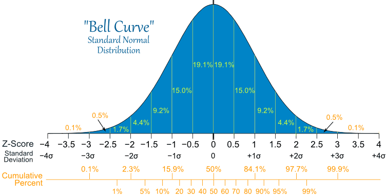
This value of z would be a random sample from the standard normal distribution, which is the distribution of z if the null hypothesis is true.
The observed value of z=43.75 corresponds to an extreme outlier p-value on the standard normal distribution curve, much less than 0.1 percent.
The p-value is the area under the curve, to the right of the value of 3.75 on the preceding normal distribution curve.
This suggests that it would be highly unlikely for us to obtain the observed value of the test statistic if we were sampling from a standard normal distribution.
We can look up the actual p-value using Python by using the scipy.stats package as follows:
In [104]: 1 - stats.norm.cdf(3.75)
Out[104]: 8.841728520081471e-05
Therefore, , that is, if the test statistic was normally distributed, then the probability to obtain the observed value is 8.8e-05, which is close to zero. So, it would be almost impossible to obtain the value that we observe if the null hypothesis was actually true.
In more formal terms, we would normally define a threshold or alpha value and reject the null hypothesis if the p-value ≤ α or fail to reject otherwise.
The typical values for α are 0.05 or 0.01. Following list explains the different values of alpha:
- p-value <0.01: There is VERY strong evidence against H0
- 0.01 < p-value < 0.05: There is strong evidence against H0
- 0.05 < p-value < 0.1: There is weak evidence against H0
- p-value > 0.1: There is little or no evidence against H0
Therefore, in this case, we would reject the null hypothesis and give credence to Intelligenza's claim and state that their claim is highly significant. The evidence against the null hypothesis in this case is significant. There are two methods that we use to determine whether to reject the null hypothesis:
- The p-value approach
- The rejection region approach
The approach that we used in the preceding example was the latter one.
The smaller the p-value, the less likely it is that the null hypothesis is true. In the rejection region approach, we have the following rule:
If , reject the null hypothesis, else retain it.
The z-test is most useful when the standard deviation of the population is known. However, in most real-world cases, this is an unknown quantity. For these cases, we turn to the t-test of significance.
For the t-test, given that the standard deviation of the population is unknown, we replace it by the standard deviation, s, of the sample. The standard error of the mean now becomes as follows:
The standard deviation of the sample s is calculated as follows:
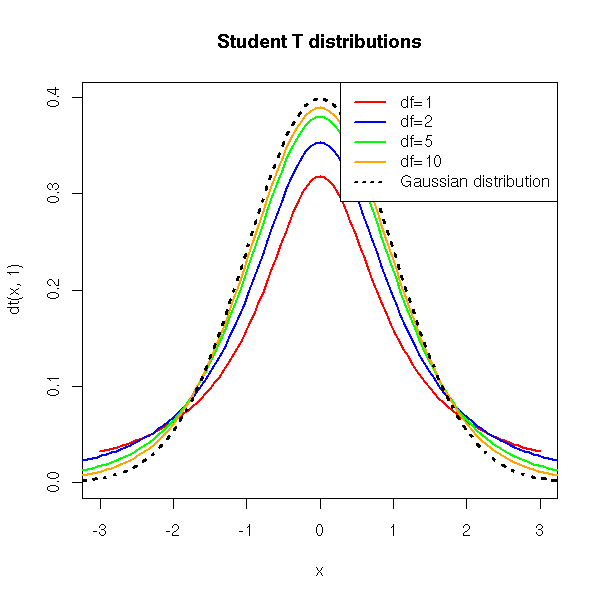
The denominator is N-1 and not N. This value is known as the number of degrees of freedom. I will now state without explanation that by the CLT the t-distribution approximates the normal, Guassian, or z-distribution as N and hence N-1 increases, that is, with increasing degrees of freedom (df). When df = ∞, the t-distribution is identical to the normal or z-distribution. This is intuitive since as df increases, the sample size increases and s approaches , the true standard deviation of the population. There are an infinite number of t-distributions, each corresponding to a different value of df.
This can be seen in the following figure:
The reference of this image is from: http://zoonek2.free.fr/UNIX/48_R/g593.png.
A more detailed technical explanation on the relationship between t-distribution, z-distribution, and the degrees of freedom can be found at http://en.wikipedia.org/wiki/Student's_t-distribution.
There are various types of t-tests. Following are the most common ones; they typically formulate a null hypothesis that makes a claim about the mean of a distribution:
- One sample independent t-test: This is used to compare the mean of a sample with that of a known population mean or known value. Let's assume that we're health researchers in Australia who are concerned about the health of the aboriginal population and wish to ascertain whether babies born to low-income aboriginal mothers have lower birth weight than is normal.
An example of a null hypothesis test for a one-sample t-test would be this: the mean birth weight for our sample of 150 deliveries of full-term, live baby deliveries from low-income aboriginal mothers is no different from the mean birth weight of babies in the general Australian population, that is, 3,367 grams.
The reference of this information is: http://bit.ly/1KY9T7f.
- Independent samples t-tests: This is used to compare means from independent samples with each other. An example of an independent sample t-test would be a comparison of fuel economy of automatic transmission versus manual transmission vehicles. This is what our real-world example will focus on.
The null hypothesis for the t-test would be this: there is no difference between the average fuel efficiency of cars with manual and automatic transmissions in terms of their average combined city/highway mileage.
- Paired samples t-test: In a paired/dependent samples t-test, we take each data point in one sample and pair it with a data point in the other sample in a meaningful way. One way to do this would be to measure against the same sample at different points in time. An example of this would be to examine the efficacy of a slimming diet by comparing the weight of a sample of participants before and after the diet.
The null hypothesis in this case would be this: there is no difference between the mean weights of participants before and after going on the slimming diet, or, more succinctly, the mean difference between paired observations is zero.
The reference for this information can be found at http://en.wikiversity.org/wiki/T-test.
In simplified terms, to do Null Signifcance Hypothesis Testing (NHST), we need to do the following:
- Formulate our null hypothesis. The null hypothesis is our model of the system, assuming that the effect we wish to verify was actually due to chance.
- Calculate our p-value.
- Compare the calculated p-value with that of our alpha, or threshold value, and decide whether to reject or accept the null hypothesis. If the p-value is low enough (lower than alpha), we will draw the conclusion that the null hypothesis is likely to be untrue.
For our real-world illustration, we wish to investigate whether manual transmission vehicles are more fuel efficient than automatic transmission vehicles. In order to do this, we will make use of the Fuel Economy data published by the US government for 2014 at http://www.fueleconomy.gov.
In [53]: import pandas as pd
         import numpy as np
         feRawData = pd.read_csv('2014_FEGuide.csv')

In [54]: feRawData.columns[:20]
Out[54]: Index([u'Model Year', u'Mfr Name', u'Division', u'Carline', u'Verify Mfr Cd', u'Index (Model Type Index)', u'Eng Displ', u'# Cyl', u'Trans as listed in FE Guide (derived from col AA thru AF)', u'City FE (Guide) - Conventional Fuel', u'Hwy FE (Guide) - Conventional Fuel', u'Comb FE (Guide) - Conventional Fuel', u'City Unadj FE - Conventional Fuel', u'Hwy Unadj FE - Conventional Fuel', u'Comb Unadj FE - Conventional Fuel', u'City Unrd Adj FE - Conventional Fuel', u'Hwy Unrd Adj FE - Conventional Fuel', u'Comb Unrd Adj FE - Conventional Fuel', u'Guzzler? ', u'Air Aspir Method'], dtype='object')

In [51]: feRawData = feRawData.rename(columns={'Trans as listed in FE Guide (derived from col AA thru AF)' :'TransmissionType',
                                               'Comb FE (Guide) - Conventional Fuel' : 'CombinedFuelEcon'})

In [57]: transType=feRawData['TransmissionType']
         transType.head()
Out[57]: 0      Auto(AM7)
         1     Manual(M6)
         2      Auto(AM7)
         3     Manual(M6)
         4    Auto(AM-S7)
         Name: TransmissionType, dtype: object
Now, we wish to modify the preceding series so that the values just contain the Auto and Manual strings . We can do this as follows:
In [58]: transTypeSeries = transType.str.split('(').str.get(0)
         transTypeSeries.head()
Out[58]: 0      Auto
         1    Manual
         2      Auto
         3    Manual
         4      Auto
         Name: TransmissionType, dtype: object
We now create a final modified DataFrame from a Series that consists of the transmission type and the combined fuel economy figures:
In [61]: feData=pd.DataFrame([transTypeSeries,feRawData['CombinedFuelEcon']]).T
         feData.head()
Out[61]:    TransmissionType    CombinedFuelEcon
         0  Auto                16
         1  Manual              15
         2  Auto                16
         3  Manual              15
         4  Auto                17
         5 rows × 2 columns
We can now separate the data for vehicles with automatic transmission from those with manual transmission as follows:
In [62]: feData_auto=feData[feData['TransmissionType']=='Auto']
         feData_manual=feData[feData['TransmissionType']=='Manual']
In [63]: feData_auto.head()
Out[63]:   TransmissionType     CombinedFuelEcon
        0  Auto                 16
        2  Auto                 16
        4  Auto                 17
        6  Auto                 16
        8  Auto                 17
        5 rows × 2 columns
This shows that there were 987 vehicles with automatic transmission versus 211 with manual transmission:
In [64]: len(feData_auto)
Out[64]: 987

In [65]: len(feData_manual)
Out[65]: 211

In [87]: np.mean(feData_auto['CombinedFuelEcon'])
Out[87]: 22.173252279635257

In [88]: np.mean(feData_manual['CombinedFuelEcon'])
Out[88]: 25.061611374407583

In [84]: import scipy.stats as stats
         stats.ttest_ind(feData_auto['CombinedFuelEcon'].tolist(),
                         feData_manual['CombinedFuelEcon'].tolist())
Out[84]: (array(-6.5520663209014325), 8.4124843426100211e-11)

In [86]: stats.ttest_ind(feData_auto['CombinedFuelEcon'].tolist(),
                         feData_manual['CombinedFuelEcon'].tolist(),
                         equal_var=False)
Out[86]: (array(-6.949372262516113), 1.9954143680382091e-11)
In this section, we will address the issue of confidence intervals. A confidence interval enables us to make a probabilistic estimate of the value of the mean of a population's given sample data.
This estimate, called an interval estimate, consists of a range of values (intervals) that act as good estimates of the unknown population parameter.
The confidence interval is bounded by confidence limits. A 95 percent confidence interval is defined as an interval in which the interval contains the population mean with 95 percent probability. So, how do we construct a confidence interval?
Suppose we have a 2-tailed t-test and we wish to construct a 95 percent confidence interval. In this case, we want the sample t-value, , corresponding to the mean to satisfy the following inequality:
Given that , which we can substitute in the preceding inequality relation to obtain this:
The interval is our 95 percent confidence interval.
Generalizing, any confidence interval for any percentage y can be expressed as , where
is the t-tailed value of
, that is,
corresponding to the desired confidence interval for y.
We will now take the opportunity to illustrate how we can calculate the confidence interval using a dataset from the popular statistical environment R. The stats models' module provides access to the datasets that are available in the core datasets package of R via the get_rdataset function.
We will consider the dataset known as faithful that consists of data obtained by observing the eruptions of the Old Faithful geyser in the Yellowstone National Park in the U.S. The two variables in the dataset are eruptions, which are the length of time the geyser erupts and waiting which is the time interval until the next eruption. There were 272 observations.
In [46]: import statsmodels.api as sma
         faithful=sma.datasets.get_rdataset("faithful")
         faithful
Out[46]: <class 'statsmodels.datasets.utils.Dataset'>

In [48]: faithfulDf=faithful.data
         faithfulDf.head()
Out[48]:    eruptions   waiting
        0   3.600       79
        1   1.800       54
        2   3.333       74
        3   2.283       62
        4  4.533        85
5 rows × 2 columns

In [50]: len(faithfulDf)
Out[50]: 272
Let us calculate a 95 percent confidence interval for the mean waiting time of the geyser. To do this, we first obtain the sample mean and standard deviation of the data:
In [80]: mean,std=(np.mean(faithfulDf['waiting']),
                   np.std(faithfulDf['waiting']))
We now make use of the scipy.stats package to calculate the confidence interval:
In [81]: from scipy import statsN=len(faithfulDf['waiting'])
        ci=stats.norm.interval(0.95,loc=mean,scale=std/np.sqrt(N))
In [82]: ci
Out[82]: (69.28440107709261, 72.509716569966201)
Thus, we can state that with 95 percent confidence that the [69.28, 72.51] interval contains the actual mean waiting time of the geyser.
Reference for this information: http://statsmodels.sourceforge.net/devel/datasets/index.html and http://docs.scipy.org/doc/scipy-0.14.0/reference/generated/scipy.stats.norm.html.
One of the most common tasks in statistics in determining the relationship between two variables is whether there is dependence between them. Correlation is the general term we use in statistics for variables that express dependence with each other.
We can then use this relationship to try and predict the value of one set of variables from the other; this is termed as regression.
The statistical dependence expressed in a correlation relationship does not imply a causal relationship between the two variables; the famous line on this is "Correlation does not imply Causation". Thus, correlation between two variables or datasets implies just a casual rather than a causal relationship or dependence. For example, there is a correlation between the amount of ice cream purchased on a given day and the weather.
For more information on correlation and dependency, refer to http://en.wikipedia.org/wiki/Correlation_and_dependence.
The correlation measure, known as correlation coefficient, is a number that captures the size and direction of the relationship between the two variables. It can vary from -1 to +1 in direction and 0 to 1 in magnitude. The direction of the relationship is expressed via the sign, with a + sign expressing positive correlation and a - sign negative correlation. The higher the magnitude, the greater the correlation with a one being termed as the perfect correlation.
The most popular and widely used correlation coefficient is the Pearson product-moment correlation coefficient, known as r. It measures the linear correlation or dependence between two x and y variables and takes values between -1 and +1.
The sample correlation coefficient r is defined as follows:
This can also be written as follows:
Here, we have omitted the summation limits.
As mentioned earlier, regression focuses on using the relationship between two variables for prediction. In order to make predictions using linear regression, the best-fitting straight line must be computed.
If all the points (values for the variables) lie on a straight line, then the relationship is deemed perfect. This rarely happens in practice and the points do not all fit neatly on a straight line. Then the relationship is imperfect. In some cases, a linear relationship only occurs among log-transformed variables. This is a log-log model. An example of such a relationship would be a power law distribution in physics where one variable varies as a power of another.
Thus, an expression such as results in the
linear relationship.
For more information see: http://en.wikipedia.org/wiki/Power_law
To construct the best-fit line, the method of least squares is used. In this method, the best-fit line is the optimal line that is constructed between the points for which the sum of the squared distance from each point to the line is the minimum. This is deemed to be the best linear approximation of the relationship between the variables we are trying to model using the linear regression. The best-fit line in this case is called the Least Squares Regression Line.
More formally, the least squares regression line is the line that has the minimum possible value for the sum of squares of the vertical distance from the data points to the line. These vertical distances are also known as residuals.
Thus, by constructing the least-squares regression line, we're trying to minimize the following expression:
We will now illustrate all the preceding points with an example. Suppose we're doing a study in which we would like to illustrate the effect of temperature on how often crickets chirp. Data for this example is obtained from a book The Song of Insects, George W Pierce in 1948. George Pierce measured the frequency of chirps made by a ground cricket at various temperatures.
We wish to investigate the frequency of cricket chirps and the temperature as we suspect that there is a relationship. The data consists of 16 data points and we read it into a data frame:
In [38]: import pandas as pd
         import numpy as np
         chirpDf= pd.read_csv('cricket_chirp_temperature.csv')
In [39]: chirpDf
Out[39]:chirpFrequency  temperature
0       20.000000       88.599998
1       16.000000       71.599998
2       19.799999       93.300003
3       18.400000       84.300003
4       17.100000       80.599998
5       15.500000       75.199997
6       14.700000       69.699997
7       17.100000       82.000000
8       15.400000       69.400002
9       16.200001       83.300003
10      15.000000       79.599998
11      17.200001       82.599998
12      16.000000       80.599998
13      17.000000       83.500000
14      14.400000       76.300003
15 rows × 2 columns
As a start, let us do a scatter plot of the data along with a regression line or line of best fit:
In [29]: plt.scatter(chirpDf.temperature,chirpDf.chirpFrequency,
            marker='o',edgecolor='b',facecolor='none',alpha=0.5)
           plt.xlabel('Temperature')
           plt.ylabel('Chirp Frequency')
           slope, intercept = np.polyfit(chirpDf.temperature,chirpDf.chirpFrequency,1)
           plt.plot(chirpDf.temperature,chirpDf.temperature*slope + intercept,'r')
           plt.show()
From the plot, we can see that there seems to be a linear relationship between temperature and the chirp frequency. We can now proceed to investigate further by using the statsmodels.ols (ordinary least squares) method to:
[37]: chirpDf= pd.read_csv('cricket_chirp_temperature.csv')
      chirpDf=np.round(chirpDf,2)
      result=sm.ols('temperature ~ chirpFrequency',chirpDf).fit()
      result.summary()

Out[37]: OLS Regression Results
   Dep. Variable: temperature     R-squared:      0.697
   Model: OLS     Adj. R-squared: 0.674
   Method:        Least Squares   F-statistic:    29.97
   Date:  Wed, 27 Aug 2014     Prob (F-statistic):     0.000107
   Time:  23:28:14        Log-Likelihood: -40.348
   No. Observations:      15      AIC:    84.70
   Df Residuals:  13      BIC:    86.11
   Df Model:      1
                   coef     std err t     P>|t| [95.0% Conf. Int.]
   Intercept     25.2323 10.060  2.508 0.026 3.499 46.966
   chirpFrequency 3.2911  0.601  5.475 0.000 1.992 4.590

   Omnibus:        1.003   Durbin-Watson:  1.818
   Prob(Omnibus):  0.606   Jarque-Bera (JB):       0.874
   Skew:   -0.391  Prob(JB):       0.646
   Kurtosis:       2.114   Cond. No.       171.
We will ignore most of the preceding results, except for the R-squared, Intercept, and chirpFrequency values.
From the preceding result, we can conclude that the slope of the regression line is 3.29, and the intercept on the temperature axis is 25.23. Thus, the regression line equation looks like this: temperature = 25.23 + 3.29 * chirpFrequency.
This means that as the chirp frequency increases by one, the temperature increases by about 3.29 degrees Fahrenheit. However, note that the intercept value is not really meaningful as it is outside the bounds of the data. We can also only make predictions for values within the bounds of the data. For example, we cannot predict what the chirpFrequency is at 32 degrees Fahrenheit as it is outside the bounds of the data; moreover, at 32 degrees Fahrenheit, the crickets would have frozen to death. The value of R, the correlation coefficient, is given as follows:
In [38]: R=np.sqrt(result.rsquared)
         R
Out[38]: 0.83514378678237422
Thus, our correlation coefficient is R = 0.835. This would indicate that about 84 percent of the chirp frequency can be explained by the changes in temperature.
Reference of this information: The Song of Insects http://www.hup.harvard.edu/catalog.php?isbn=9780674420663
The data is sourced from http://bit.ly/1MrlJqR.
For a more in-depth treatment of single and multi-variable regression, refer to the following websites:
- Regression (Part I): http://bit.ly/1Eq5kSx
- Regression (Part II): http://bit.ly/1OmuFTV