10 • • • • • • • • • • • • • • • • • • • • • • •
A Pretty Mathematical Face
HOW WOULD YOU DESCRIBE YOUR facial appearance? Granted, it may depend how long ago you awoke and if you have had your morning shower or coffee. Still, would you consider yourself a cross between Tom Cruise, Audrey Hepburn, and Clark Gable, or Robert Downey Jr. and Ellen DeGeneres? Let’s see how mathematics can help answer such questions.
We’ll work with a library of grayscale images of the 16 famous people seen in Figure 10.1. Our goal will be to find the combination of these pictures that best approximates a target image.
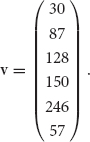
Recall from earlier in the book that the grayscale information of the image in Figure 10.2 can be stored in the following matrix:
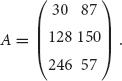
Recall also that our grayscale values are all integers from 0 to 255 where 0 is black and 255 is white.
In this chapter, we will store the grayscale information in a vector. So the image information for Figure 10.2 would be stored in a vector:
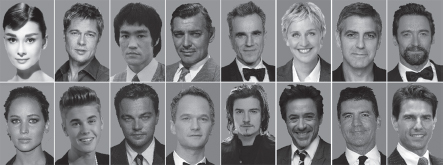
Figure 10.1. Library of famous faces used in facial recognition.

Figure 10.2. Visualizing the grayscale data contained in a matrix.
Given that our 16 library images and 1 target image are vectors, we want to find the combination of the library images that satisfies the linear system:
![]()
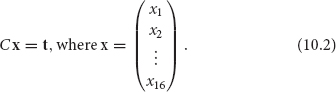
where ci and t are the vectors storing image information for the ith library photo and the target image, respectively. The numbers x1, x2, … x16 give us the amount of the corresponding image to add into the sum.
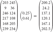
Let’s look at a small example. Suppose x1 = 0.25 and x2 = 0.61, and our vectors are
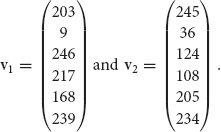
The vectors v1 and v2 correspond to the images in Figure 10.3 (a) and (b). We can now form our target image,
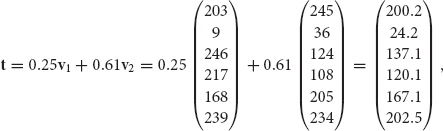
which corresponds to the image in Figure 10.3 (c).
In equation 10.1, the variables x1, x2, …, x16 are the unknowns. Let’s express this system of equations in another form by creating the matrix C where the first column of C equals c1, the second column of C equals c2 and so forth. We will solve the same problem as equation 10.1 if we solve the linear system:
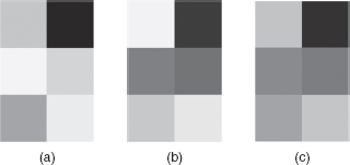
Figure 10.3. The grayscale image in (c) is a weighted sum of the image information in (a) and (b).
We can see this from our earlier example since
ORIGINS OF MATRIX METHODS
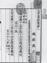
The Jiuzhang Suanshu is a Chinese manuscript dating from approximately 200 BC and containing 246 problems intended to illustrate methods of solution for everyday problems in areas such as engineering, surveying, and trade. (To the left, we see the opening of Chapter 1.) Chapter 8 of this ancient document details the first known example of matrix methods with a method known as fangcheng, which is what would become known centuries later as Gaussian elimination. [21, 2]
Chances are that there does not exist a combination of the library of images that can exactly replicate the target image. So, we cannot attain equality in the linear system in equation 10.2. Instead, we’ll solve
![]()
What is meant by that approximation symbol? In terms of our library images, we want to find the sum that “best” approximates the target image. Mathematically, we will choose x by looking at the vector r = t−Cx. The first thing to notice about r is that it will equal 0 if there exists a combination of the images that produces the target; that is, Cx = t. In all other cases, we will choose the vector x that minimizes the length of r.
A Collection of Stars
Getting more personal, let’s find a linear combination of the library images that best approximates the following picture of the author. Which celebrity do you think will be used most (least) in the construction of my photo?

The dimensions of this photo are 600 × 900 pixels. Each celebrity photo has the same dimensions. So, we are interested in solving:
![]()
where C is a 540, 000 × 16 matrix, x is a 16 × 1 vector and t is a 540, 000 × 1 vector. That’s a lot of numbers, so a computer will be helpful! Our goal is succinctly stated as choosing x that minimizes the length of the residual vector r. How do we find the vector x that produces this minimal length among the infinite possible values for the entries of x?
One approach is to solve the linear system
![]()
It may be surprising that solving this equation produces our desired x among the infinite number of possibilities. Why does it work? It’s a bit beyond the scope of this book to unveil the theory behind why this is true. You may want to look it up. This method is called a least squares problem. The theory behind this approach to finding the solution, while requiring only a few lines of mathematics, involves taking the derivatives of the linear system Cx = t with respect to the elements of the vector x.
It turns out that solving equation 10.3 isn’t actually the best method for solving such a problem on a computer. It can lead to considerable round-off error. A more reliable answer results from a method that involves the computation of a matrix decomposition. Such a method produced the results of this chapter.
So, for my image what combination of photos in the library produces the best result? See the results in Table 10.1.
TABLE 10.1.
Weights of the celebrity photos for the author’s image.
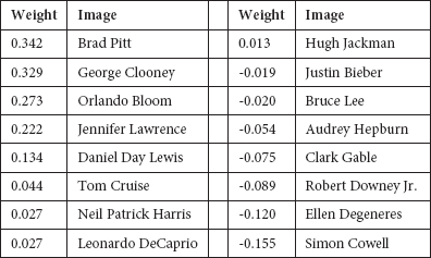
Notice that the celebrities with the highest weights to produce an approximation to my image are Brad Pitt, George Clooney, and Orlando Bloom, all of whom have been named People Magazine’s Sexiest Man Alive. I must say that I’m pretty pleased with the results coming from that residual vector of minimal length! Notice the next highest weight, Jennifer Lawrence, is given a weight just less than that of Orlando Bloom. Moreover, notice how several celebrities have negative weights, which corresponds to the contents of such pictures being subtracted in the sum of the images. So, the best approximation to my picture actually involves subtracting out 0.155 of Simon Cowell’s image.
Why were such choices made? Keep in mind that we are approximating the solution to a linear system and not really facial features. The algorithm isn’t trying to match noses or eyes. It simply matches, as best it can, numbers in a vector that result from matrix-vector multiplication. As such, the placement of the image plays an important role in the outcome. To see this, let’s shift my image down slightly as seen in Figure 10.4. Now, the top 4 weights of the celebrity photos can be seen in Table 10.2. Note how Justin Bieber jumped from a negative weight for the image in Figure 10.4 (a) to the third highest weight. Further, my “connection” with George Clooney is lost at least in the top 4 celebrity weights.
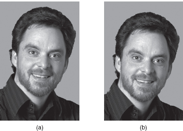
Figure 10.4. The image in (a) is slightly shifted to create image (b).
TABLE 10.2.
Weights for the top 4 celebrity photos to create the best approximation of the author’s image in Figure 10.4 (b).
Weight |
Image |
0.351 |
Brad Pitt |
0.279 |
Orlando Bloom |
0.154 |
Justin Bieber |
0.134 |
Jennifer Lawrence |
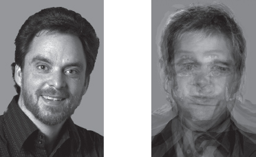
Figure 10.5. The original image (left) and the best approximation (right) using a library of 16 celebrity photos.
To further see why the rankings are as they are, it helps to see the image that results from our approximation. In Figure 10.5, we see the best approximation (right) to the author’s image (left). Notice how the author’s hair and dark shirt appear to be fairly well approximated. With this in mind, look carefully at the images of Brad Pitt, George Clooney, Orlando Bloom, and Jennifer Lawrence in our library of photos. It may be easier to see why such stars topped the list.
Can we get a better image that is closer to the author’s likeness? Probably but it would require more photos. Further, the images in our library differ in a variety of attributes such as the orientation of the face. How can we find more uniform libraries of faces? It is relatively easy as databases for facial recognition exist; some are free and others require a fee. You may want to use a search engine to find such resources. One of which is the Yale Face Database, which contains 5760 single light source images of 10 subjects each seen under 576 viewing conditions (9 poses x 64 illumination conditions). Such databases generally do not have celebrities as their subjects and would not enable you to describe your appearance in terms of a combination of famous faces. For instance, I could now describe myself as a combination of Brad Pitt, George Clooney, Orlando Bloom, and, yes, Jennifer Lawrence.
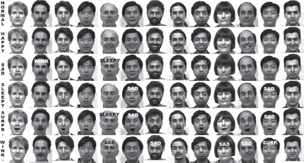
Figure 10.6. Faces from the Yale Face Database.
A more common method in facial recognition uses principle component analysis. Such an approach utilizes the eigenvectors of the covariance matrix resulting from the library of images and generally involves a library of several thousand images. In this context, the eigenvectors of the covariance matrix are often referred to as eigenfaces. We see such a set of eigenfaces for our library of celebrities in Figure 10.7.
Celebrity in Disguise
Let’s change gears for a moment and disguise our celebrity. In particular, George Clooney decides to disguise himself with Hugh Jackman’s goatee as seen in Figure 10.8 (left). Using this disguised image as our target image, what linear combination results from the library of celebrity images? Our algorithm chooses the following top 4 weights to produce the best approximation seen in Figure 10.8 (right).
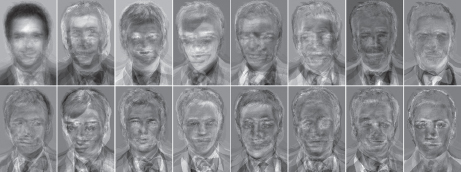
Figure 10.7. Eigenfaces for our library of famous faces.
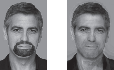
Figure 10.8. A disguised George Clooney (left) and our algorithm’s approximation (right).
Weight |
Image |
0.810 |
George Clooney |
0.127 |
Hugh Jackman |
0.086 |
Leonardo DeCaprio |
0.079 |
Brad Pitt |
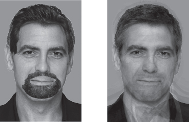
Wanting to be more mathematically incognito, suppose Clooney adds a toupee resembling Hugh Jackman’s hairstyle. Can he fool our program now? In Figure 10.9, you see our algorithm’s approximation (right) to the original image (left); what do you think?
While our algorithm’s best approximation does indeed pick up the increased Jackman-ness of the photo, it still recognizes the dominant contributions of Clooney’s photo. This is reflected numerically by the top 4 weights in the following table.
Weight |
Image |
0.743 |
George Clooney |
0.156 |
Hugh Jackman |
0.117 |
Tom Cruise |
0.101 |
Leonardo DeCaprio |
George Clooney will need to do better to fool our algorithm! Note, you could use this technique on your photo. You could, as with my photo, see what stars best approximate your image. If you want to change the results, alter your image with a new haircut, for instance, and see if you find a celebrity combination to your liking. In this sense, you can preview any potential mathematical makeover.
To end the chapter, here are two problems, from the Jiuzhang Suanshu, mentioned earlier in the chapter. Here’s the first:
There are three classes of grain, of which three bundles of the first class, two of the second, and one of the third make 39 measures. Two of the first, three of the second and, one of the third make 34 measures. And one of the first, two of the second and three of the third make 26 measures. How many measures of grain are contained in one bundle of each class?
For this second problem write the associated linear system with five equations and six unknowns corresponding to this problem. The linear systems we solved in this chapter had no solution, which is why we used least squares. This puzzle has infinitely many solutions. Find the smallest solution in which the lengths are positive integers for the following problem from the ancient Chinese text.
There are five families which share a well. 2 of A’s ropes are short of the well’s depth by 1 of B’s ropes. 3 of B’s ropes are short of the depth by 1 of C’s ropes. 4 of C’s ropes are short by 1 of D’s ropes. 5 of D’s ropes are short by 1 of E’s ropes. 6 of E’s ropes are short by 1 of A’s ropes. Find the depth of the well and the length of each rope.
Challenge 10.1. Find the solution to both of these problems from the Jiuzhang Suanshu.