
11
GRADIENT DESCENT
In this final chapter, we’ll slow down a bit and consider gradient descent afresh. We’ll begin by reviewing the idea of gradient descent using illustrations, discussing what it is and how it works. Next, we’ll explore the meaning of stochastic in stochastic gradient descent. Gradient descent is a simple algorithm that invites tweaking, so after we explore stochastic gradient descent, we’ll consider a useful and commonly used tweak: momentum. We’ll conclude the chapter by discussing more advanced, adaptive gradient descent algorithms, specifically RMSprop, Adagrad, and Adam.
This is a math book, but gradient descent is very much applied math, so we’ll learn by experimentation. The equations are straightforward, and the math we saw in previous chapters is relevant as background. Therefore, consider this chapter an opportunity to apply what we’ve learned so far.
The Basic Idea
We’ve encountered gradient descent several times already. We know the form of the basic gradient descent update equations from Equation 10.14:

Here, ΔW and Δb are errors based on the partial derivatives of the weights and biases, respectively; η (eta) is a step size or learning rate, a value we use to adjust how we move.
Equation 11.1 isn’t specific to machine learning. We can use the same form to implement gradient descent on arbitrary functions. Let’s discuss gradient descent using 1D and 2D examples to lay a foundation for how it operates. We’ll use an unmodified form of gradient descent known as vanilla gradient descent.
Gradient Descent in One Dimension
Let’s begin with a scalar function of x:
Equation 11.2 is a parabola facing upward. Therefore, it has a minimum. Let’s find the minimum analytically by setting the derivative to zero and solving for x:
The minimum of the parabola is at x = 1. Now, let’s instead use gradient descent to find the minimum of Equation 11.2. How should we begin?
First, we need to write the proper update equation, the form of Equation 11.1 that applies in this case. We need the gradient, which for a 1D function is simply the derivative, f′(x) = 12x − 12. With the derivative, gradient descent becomes
Notice that we subtract η (12x − 12). This is why the algorithm is called gradient descent. Recall that the gradient points in the direction of maximum change in the function’s value. We’re interested in minimizing the function, not maximizing it, so we move in the direction opposite to the gradient toward smaller function values; therefore, we subtract.
Equation 11.3 is one gradient descent step. It moves from an initial position, x, to a new position based on the value of the slope at the current position. Again η, the learning rate, governs how far we move.
Now that we have the equation, let’s implement gradient descent. We’ll plot Equation 11.2, pick a starting position, say x = −0.9, and iterate Equation 11.3, plotting the function value at each new position of x. If we do this, we should see a series of points on the function that move ever closer to the minimum position at x = 1. Let’s write some code.
First, we implement Equation 11.2 and its derivative:
def f(x):
return 6*x**2 - 12*x + 3
def d(x):
return 12*x - 12
Next, we plot the function, and then we iterate Equation 11.3, plotting the new pair, (x, f(x)), each time:
import numpy as np
import matplotlib.pylab as plt
❶ x = np.linspace(-1,3,1000)
plt.plot(x,f(x))
❷ x = -0.9
eta = 0.03
❸ for i in range(15):
plt.plot(x, f(x), marker='o', color='r')
❹ x = x - eta * d(x)
Let’s walk through the code. After importing NumPy and Matplotlib, we plot Equation 11.2 ❶. Next, we set our initial x position ❷ and take 15 gradient descent steps ❸. We plot before stepping, so we see the initial x but do not plot the last step, which is fine in this case.
The final line ❹ is key. It implements Equation 11.3. We update the current x position by multiplying the derivative’s value at x by η = 0.03 as the step size. The code above is in the file gd_1d.py. If we run it, we get Figure 11-1.
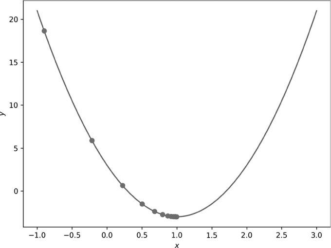
Figure 11-1: Gradient descent in one dimension with small steps (η = 0.03)
Our initial position, which we can think of as an initial guess at the location of the minimum, is x = −0.9. Clearly, this isn’t the minimum. As we take gradient descent steps, we move successively closer to the minimum, as the sequence of circles moving toward it shows.
Notice two things here. First, we do get closer and closer to the minimum. After 14 steps, we are, for all intents and purposes, at the minimum: x = 0.997648. Second, each gradient descent step leads to smaller and smaller changes in x. The learning rate is constant at η = 0.03, so the source of the smaller updates to x must be smaller and smaller values of the derivative at each x position. This makes sense if we think about it. As we approach the minimum position, the derivative gets smaller and smaller, until it reaches zero at the minimum, so the update using the derivative gets successively smaller as well.
We selected the step size for Figure 11-1 to move smoothly toward the minimum of the parabola. What if we change the step size? Further along in gd_1d.py, the code repeats the steps above, starting at x = 0.75 and setting η = 0.15 to take steps that are five times larger than those plotted in Figure 11-1. The result is Figure 11-2.
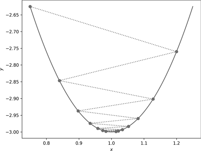
Figure 11-2: Gradient descent in one dimension with large steps (η = 0.15)
In this case, the steps overshoot the minimum. The new x positions oscillate, bouncing back and forth over the true minimum position. The dashed lines connect successive x positions. The overall search still approaches the minimum but takes longer to reach it, as the large step size makes each update to x tend to move past the minimum.
Small gradient descent steps move short distances along the function, whereas large steps move large distances. If the learning rate is too small, many gradient descent steps are necessary. If the learning rate is too large, the search overshoots and oscillates around the minimum position. The proper learning rate is not immediately obvious, so intuition and experience come into play when selecting it. Additionally, these examples fixed η. There’s no reason why η has to be a constant. In many deep learning applications, the learning rate is not constant but evolves as training progresses, effectively making η a function of the number of gradient descent steps taken.
Gradient Descent in Two Dimensions
Gradient descent in one dimension is straightforward enough. Let’s move to two dimensions to increase our intuition about the algorithm. The code referenced below is in the file gd_2d.py. We’ll first consider the case where the function has a single minimum, then look at cases with multiple minima.
Gradient Descent with a Single Minimum
To work in two dimensions, we need a scalar function of a vector, f(x) = f(x, y), where, to make it easier to follow, we separate the vector into its components, x = (x, y).
The first function we’ll work with is
f(x, y) = 6x2 + 9y2 − 12x − 14y + 3
To implement gradient descent, we need the partial derivatives as well:
Our update equations become
In code, we define the function and partial derivatives:
def f(x,y):
return 6*x**2 + 9*y**2 - 12*x - 14*y + 3
def dx(x):
return 12*x - 12
def dy(y):
return 18*y - 14
Since the partial derivatives are independent of the other variable, we get away with passing only x or y. We’ll see an example later in this section where that’s not the case.
Gradient descent follows the same pattern as before: select an initial position, this time a vector, iterate for some number of steps, and plot the path. The function is 2D, so we first plot it using contours, as shown next.
N = 100
x,y = np.meshgrid(np.linspace(-1,3,N), np.linspace(-1,3,N))
z = f(x,y)
plt.contourf(x,y,z,10, cmap="Greys")
plt.contour(x,y,z,10, colors='k', linewidths=1)
plt.plot([0,0],[-1,3],color='k',linewidth=1)
plt.plot([-1,3],[0,0],color='k',linewidth=1)
plt.plot(1,0.7777778,color='k',marker='+')
This code requires some explanation. To plot contours, we need a representation of the function over a grid of (x, y) pairs. To generate the grid, we use NumPy, specifically np.meshgrid. The arguments to np.meshgrid are the x and y points, here provided by np.linspace, which itself generates a vector from −1 to 3 of N = 100 evenly spaced values. The np.meshgrid function returns two 100 × 100 matrices. The first contains the x values over the given range, and the second contains the y values. All possible (x, y) pairs are represented in the return value to form a grid of points covering the region of −1 . . . 3 in both x and y. Passing these points to the function then returns z, a 100 × 100 matrix of the function value at each (x, y) pair.
We could plot the function in 3D, but that’s difficult to see and unnecessary in this case. Instead, we’ll use the function values in x, y, and z to generate contour plots. Contour plots show 3D information as a series of lines of equal z value. Think of lines around a hill on a topographic map, where each line is at the same altitude. As the hill gets higher, the lines enclose successively smaller regions.
Contour plots come in two varieties, as either lines of equal function value or shading over ranges of the function. We’ll plot both varieties using a grayscale map. That’s the net result of calling Matplotlib’s plt.contourf and plt.contour functions. The remaining plt.plot calls show the axes and mark the function minimum with a plus sign. The contour plots are such that lighter shades imply lower function values.
We’re now ready to plot the sequence of gradient descent steps. We’ll plot each position in the sequence and connect them with a dashed line to make the path clear (see Listing 11-1). In code, that’s
x = xold = -0.5
y = yold = 2.9
for i in range(12):
plt.plot([xold,x],[yold,y], marker='o', linestyle='dotted', color='k')
xold = x
yold = y
x = x - 0.02 * dx(x)
y = y - 0.02 * dy(y)
Listing 11-1: Gradient descent in two dimensions
We begin at (x, y) = (−0.5, 2.9) and take 12 gradient descent steps. To connect the last position to the new position using a dashed line, we track both the current position in x and y and the previous position, (xold, yold). The gradient descent step updates both x and y using η = 0.02 and calling the respective partial derivative functions, dx and dy.
Figure 11-3 shows the gradient descent path that Listing 11-1 follows (circles) along with two other paths starting at (1.5, −0.8) (squares) and (2.7, 2.3) (triangles).
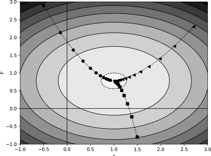
Figure 11-3: Gradient descent in two dimensions for small steps
All three gradient descent paths converge toward the minimum of the function. This isn’t surprising, as the function has only one minimum. If the function has a single minimum, then gradient descent will eventually find it. If the step size is too small, many steps might be necessary, but they will ultimately converge on the minimum. If the step size is too large, gradient descent may oscillate around the minimum but continually step over it.
Let’s change our function a bit to stretch it in the x direction relative to the y direction:
f(x, y) = 6x2 + 40y2 − 12x − 30y + 3
This function has partials ∂f/∂x = 12x − 12 and ∂f/∂y = 80y − 30.
Additionally, let’s pick two starting locations, (−0.5, 2.3) and (2.3, 2.3), and generate a sequence of gradient descent steps with η = 0.02 and η = 0.01, respectively. Figure 11-4 shows the resulting paths.

Figure 11-4: Gradient descent in 2D with larger steps and a slightly different function
Consider the η = 0.02 (circle) path first. The new function is like a canyon, narrow in y but long in x. The larger step size oscillates up and down in y as it moves toward the minimum in x. Bouncing off the canyon walls aside, we still find the minimum.
Now, take a look at the η = 0.01 (square) path. It quickly falls into the canyon and then moves slowly over the flat region along the canyon floor toward the minimum position. The component of the vector gradient (the x and y partial derivative values) along the x direction is small in the canyon, so motion along x is proportionately slow. There is no motion in the y direction—the canyon is steep, and the relatively small learning rate has already located the canyon floor, where the gradient is primarily along x.
What’s the lesson here? Again, the step size matters. However, the shape of the function matters even more. The minimum of the function lies at the bottom of a long, narrow canyon. The gradient along the canyon is tiny; the canyon floor is flat in the x direction, so motion is slow because it depends on the gradient value. We frequently encounter this effect in deep learning: if the gradient is small, learning is slow. This is why the rectified linear unit has come to dominate deep learning; the gradient is a constant one for positive inputs. For a sigmoid or hyperbolic tangent, the gradient approaches zero when inputs are far from zero.
Gradient Descent with Multiple Minima
The functions we’ve examined so far have a single minimum value. What if that isn’t the case? Let’s see what happens to gradient descent when the function has more than one minimum. Consider this function:
Equation 11.4 is the sum of two inverted Gaussians, one with a minimum value of −2 at (−1, 1) and the other with a minimum of −1 at (1, −1). If gradient descent is to find the global minimum, it should find it at (−1, 1). The code for this example is in gd_multiple.py.
The partial derivatives are

which translates into the following code:
def f(x,y):
return -2*np.exp(-0.5*((x+1)**2+(y-1)**2)) +
-np.exp(-0.5*((x-1)**2+(y+1)**2))
def dx(x,y):
return 2*(x+1)*np.exp(-0.5*((x+1)**2+(y-1)**2)) +
(x-1)*np.exp(-0.5*((x-1)**2+(y+1)**2))
def dy(x,y):
return (y+1)*np.exp(-0.5*((x-1)**2+(y+1)**2)) +
2*(y-1)*np.exp(-0.5*((x+1)**2+(y-1)**2))
Notice, in this case, the partial derivatives do depend on both x and y.
The code for the gradient descent portion of gd_multiple.py is as before. Let’s run the cases in Table 11-1.
Table 11-1: Different Starting Positions and Number of Gradient Descent Steps Taken
Starting point |
Steps |
Symbol |
|---|---|---|
(–1.5,1.2) |
9 |
circle |
(1.5,–1.8) |
9 |
square |
(0,0) |
20 |
plus |
(0.7,–0.2) |
20 |
triangle |
(1.5,1.5) |
30 |
asterisk |
The Symbol column refers to the plot symbol used in Figure 11-5. For all cases, η = 0.4.
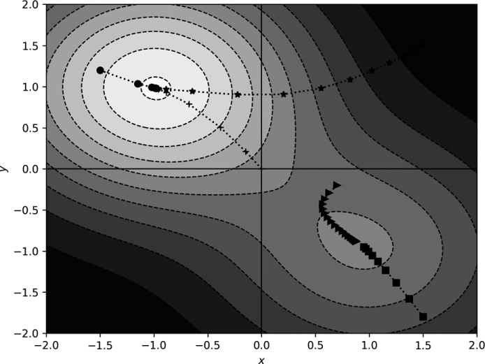
Figure 11-5: Gradient descent for a function with two minima
The gradient descent paths indicated in Figure 11-5 make sense. In three of the five cases, the path does move into the well that the deeper of the two minima defines—a successful search. However, for the triangle and the square, gradient descent fell into the wrong minimum. Clearly, how successful gradient descent is, in this case, depends on where we start the process. Once the path moves downhill to a deeper position, gradient descent has no way to escape upward to find a potentially better minimum.
Current thinking is that the loss landscape for a deep learning model contains many minima. It’s also currently believed that in most cases, the minima are pretty similar, which partially explains the success of deep learning models—to train them, you don’t need to find the one, magic, global minimum of the loss, only one of the (probably) many that are (probably) about as good as any of the others.
I selected the initial positions used for the examples in this section intentionally based on knowledge of the function’s form. For a deep learning model, picking the starting point means random initialization of the weights and biases. In general, we don’t know the form of the loss function, so initialization is a shot in the dark. Most of the time, or at least much of the time, gradient descent produces a well-performing model. Sometimes, however, it doesn’t; it fails miserably. In those cases, it’s possible the initial position was like the square in Figure 11-5: it fell into an inferior local minimum because it started in a bad place.
Now that we have a handle on gradient descent, what it is, and how it works, let’s investigate how we can apply it in deep learning.
Stochastic Gradient Descent
Training a neural network is primarily the act of minimizing the loss function while preserving generalizability via various forms of regularization. In Chapter 10, we wrote the loss as L(θ; x, y) for a vector of the weights and biases, θ (theta), and training instances (x, y), where x is the input vectors and y is the known labels. Note how here, x is a stand-in for all training data, not just a single sample.
Gradient descent needs ∂L/∂θ, which we get via backpropagation. The expression ∂L/∂θ is a concise way of referring to all the individual weight and bias error terms backpropagation gives us. We get ∂L/∂θ by averaging the error over the training data. This begs the question: Do we average over all of the training data or only some of the training data?
Passing all the training data through the model before taking a gradient descent step is called batch training. At first blush, batch training seems sensible. After all, if our training set is a good sample from the parent distribution that generates the sort of data our model intends to work with, then why not use all of that sample to do gradient descent?
When datasets were small, batch training was the natural thing to do. However, models got bigger, as did datasets, and suddenly the computational burden of passing all the training data through the model for each gradient descent step became too much. This chapter’s examples already hint that many gradient descent steps might be necessary to find a good minimum position, especially for tiny learning rates.
Therefore, practitioners began to use subsets of the training data for each gradient descent step—the minibatch. Minibatch training was probably initially viewed as a compromise, as the gradient calculated over the minibatch was “wrong” because it wasn’t based on the performance of the full training set.
Of course, the difference between batch and minibatch is just an agreed-upon fiction. In truth, it’s a continuum from a minibatch of one to a minibatch of all available samples. With that in mind, all the gradients computed during network training are “wrong,” or at least incomplete, as they are based on incomplete knowledge of the data generator and the full set of data it could generate.
Rather than a concession, then, minibatch training is reasonable. The gradient over a small minibatch is noisy compared to that computed over a larger minibatch, in the sense that the small minibatch gradient is a coarser estimate of the “real” gradient. When things are noisy or random, the word stochastic tends to show up, as it does here. Gradient descent with minibatches is stochastic gradient descent (SGD).
In practice, gradient descent using smaller minibatches often leads to models that perform better than those trained with larger minibatches. The rationale generally given is that the noisy gradient of the smaller minibatch helps gradient descent avoid falling into poor local minima of the loss landscape. We saw this effect in Figure 11-5, where the triangle and the square both fell into the wrong minimum.
Again, we find ourselves strangely fortunate. Before, we were fortunate because first-order gradient descent succeeded in training models that shouldn’t train due to nonlinear loss landscapes, and now we get a boost by intentionally using small amounts of data to estimate gradients, thereby skipping a computational burden likely to make the entire enterprise of deep learning too cumbersome to implement in many cases.
How large should our minibatch be? Minibatch size is a hyperparameter, something we need to select to train the model, but is not part of the model itself. The proper minibatch size is dataset-dependent. For example, in the extreme, we could take a gradient descent step for each sample, which sometimes works well. This case is often referred to as online learning. However, especially if we use layers like batch normalization, we need a minibatch large enough to make the calculated means and standard deviations reasonable estimates. Again, as with most everything else in deep learning at present, it’s empirical, and you need to both have intuition and try many variations to optimize the training of the model. This is why people work on AutoML systems, systems that seek to do all the hyperparameter tuning for you.
Another good question: What should be in the minibatch? That is, what small subset of the full dataset should we use? Typically, the order of the samples in the training set is randomized, and minibatches are pulled from the set as successive chunks of samples until all samples have been used. Using all the samples in the dataset defines one epoch, so the number of samples in the training set divided by the minibatch size determines the number of minibatches per epoch.
Alternatively, as we did for NN.py, a minibatch might genuinely be a random sampling from the available data. It’s possible that a particular training sample is never used while another is used many times, but on the whole, the majority of the dataset is used during training.
Some toolkits train for a specified number of minibatches. Both NN.py and Caffe operate this way. Other toolkits, like Keras and sklearn, use epochs. Gradient descent steps happen after a minibatch is processed. Larger minibatches result in fewer gradient descent steps per epoch. To compensate, practitioners using toolkits that use epochs need to ensure that the number of gradient descent steps increases as minibatch size increases—larger minibatches require more epochs to train well.
To recap, deep learning does not use full batch training for at least the following reasons:
The computational burden is too great to pass the entire training set through the model for each gradient descent step.
The gradient computed from the average loss over a minibatch is a noisy but reasonable estimate of the true, and ultimately unknowable, gradient.
The noisy gradient points in a slightly wrong direction in the loss landscape, thereby possibly avoiding bad minima.
Minibatch training simply works better in practice for many datasets.
Reason #4 should not be underestimated: many practices in deep learning are employed initially because they simply work better. Only later are they justified by theory, if at all.
As we already implemented SGD in Chapter 10 (see NN.py), we won’t reimplement it here, but in the next section, we’ll add momentum to see how that affects neural network training.
Momentum
Vanilla gradient descent relies solely on the value of the partial derivative multiplied by the learning rate. If the loss landscape has many local minima, especially if they’re steep, vanilla gradient descent might fall into one of the minima and be unable to recover. To compensate, we can modify vanilla gradient descent to include a momentum term, a term that uses a fraction of the previous step’s update. Including this momentum in gradient descent adds inertia to the algorithm’s motion through the loss landscape, thereby potentially allowing gradient descent to move past bad local minima.
Let’s define and then experiment with momentum using 1D and 2D examples, as we did earlier. After that, we’ll update our NN.py toolkit to use momentum to see how that affects models trained on more complex datasets.
What Is Momentum?
In physics, the momentum of a moving object is defined as the mass times the velocity, p = mv. However, velocity itself is the first derivative of the position, v = dx/dt, so momentum is mass times how fast the position of the object is changing in time.
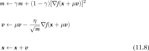
For gradient descent, position is the function value, and time is the argument to the function. The velocity, then, is how fast the function value changes with a change in the argument, ∂f/∂x. Therefore, we can think of momentum as a scaled velocity term. In physics, the scale factor is the mass. For gradient descent, the scale factor is μ (mu), a number between zero and one.
If we call the gradient including the momentum term v, then the gradient descent update equation that was
becomes
for some initial velocity, v = 0, and the “mass,” μ.
Let’s walk through Equation 11.5 to understand what it means. The two-step update, first v and then x, makes it easy to iterate, as we know we must do for gradient descent. If we substitute v into the update equation for x, we get
This makes it clear that the update includes the gradient step we had previously but adds back in a fraction of the previous step size. It’s a fraction because we restrict μ to [0, 1]. If μ = 0, we’re back to vanilla gradient descent. It might be helpful to think of μ as a scale factor, the fraction of the previous velocity to keep along with the current gradient value.
The momentum term tends to keep motion through the loss landscape heading in its previous direction. The value of μ determines the strength of that tendency. Deep learning practitioners typically use μ = 0.9, so most of the previous update direction is maintained in the next step, with the current gradient providing a small adjustment. Again, like many things in deep learning, this number was chosen empirically.
Newton’s first law of motion states that an object in motion remains in motion unless acted upon by an outside force. Resistance to an external force is related to the object’s mass and is called inertia. So, we might also view the μv term as inertia, which might have been a better name for it.
Regardless of the name, now that we have it, let’s see what it does to the 1D and 2D examples we worked through earlier using vanilla gradient descent.
Momentum in 1D
Let’s modify the 1D and 2D examples above to use a momentum term. We’ll start with the 1D case. The updated code is in the file gd_1d_momentum.py and appears here as Listing 11-2.
import matplotlib.pylab as plt
def f(x):
return 6*x**2 - 12*x + 3
def d(x):
return 12*x - 12
❶ m = ['o','s','>','<','*','+','p','h','P','D']
x = np.linspace(0.75,1.25,1000)
plt.plot(x,f(x))
❷ x = xold = 0.75
eta = 0.09
mu = 0.8
v = 0.0
for i in range(10):
❸ plt.plot([xold,x], [f(xold),f(x)], marker=m[i], linestyle='dotted',
color='r')
xold = x
v = mu*v - eta * d(x)
x = x + v
for i in range(40):
v = mu*v - eta * d(x)
x = x + v
❹ plt.plot(x,f(x),marker='X', color='k')
Listing 11-2: Gradient descent in one dimension with momentum
Listing 11-2 is a bit dense, so let’s parse it out. First, we are plotting, so we include Matplotlib. Next, we define the function, f(x), and its derivative, d(x), as we did before. To configure plotting, we define a collection of markers ❶ and then plot the function itself. As before, we begin at x = 0.75 ❷ and set the step size (eta), momentum (mu), and initial velocity (v).
We’re now ready to iterate. We’ll use two gradient descent loops. The first plots each step ❸ and the second continues gradient descent to demonstrate that we do eventually locate the minimum, which we mark with an 'X' ❹. For each step, we calculate the new velocity by mimicking Equation 11.5, and then we add the velocity to the current position to get the next position.
Figure 11-6 shows the output of gd_1d_momentum.py.
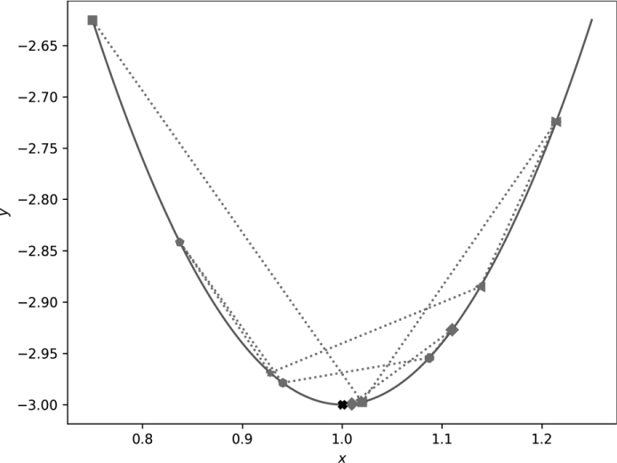
Figure 11-6: Gradient descent in one dimension with momentum
Note that we intentionally used a large step size (η), so we overshoot the minimum. The momentum term tends to overshoot minima as well. If you follow the dashed line and the sequence of plot markers, you can walk through the first 10 gradient descent steps. There is oscillation, but the oscillation is damped and eventually settles at the minimum, as marked. Adding momentum enhanced the overshoot due to the large step size. However, even with the momentum term, which isn’t advantageous here, because there’s only one minimum, with enough gradient descent steps, we find the minimum in the end.
Momentum in 2D
Now, let’s update our 2D example. We’re working with the code in gd _momentum.py. Recall that, for the 2D example, the function is the sum of two inverted Gaussians. Including momentum updates the code slightly, as shown in Listing 11-3:
def gd(x,y, eta,mu, steps, marker):
xold = x
yold = y
❶ vx = vy = 0.0
for i in range(steps):
plt.plot([xold,x],[yold,y], marker=marker,
linestyle='dotted', color='k')
xold = x
yold = y
❷ vx = mu*vx - eta * dx(x,y)
vy = mu*vy - eta * dy(x,y)
❸ x = x + vx
y = y + vy
❹ gd( 0.7,-0.2, 0.1, 0.9, 25, '>')
gd( 1.5, 1.5, 0.02, 0.9, 90, '*')
Listing 11-3: Gradient descent in two dimensions with momentum
Here, we have the new function, gd, which performs gradient descent with momentum beginning at (x,y), using the given μ and η, and runs for steps iterations.
The initial velocity is set ❶, and the loop begins. The velocity update of Equation 11.5 becomes vx = mu*vx - eta * dx(x,y) ❷, and the position update becomes x = x + vx ❸. As before, a line is plotted between the last position and the current one to track motion through the function landscape.
The code in gd_momentum.py traces the motion starting at two of the points we used before, (0.7, −0.2) and (1.5, 1.5) ❹. Note the number of steps and learning rate vary by point to keep the plot from becoming too cluttered. The output of gd_momentum.py is Figure 11-7.
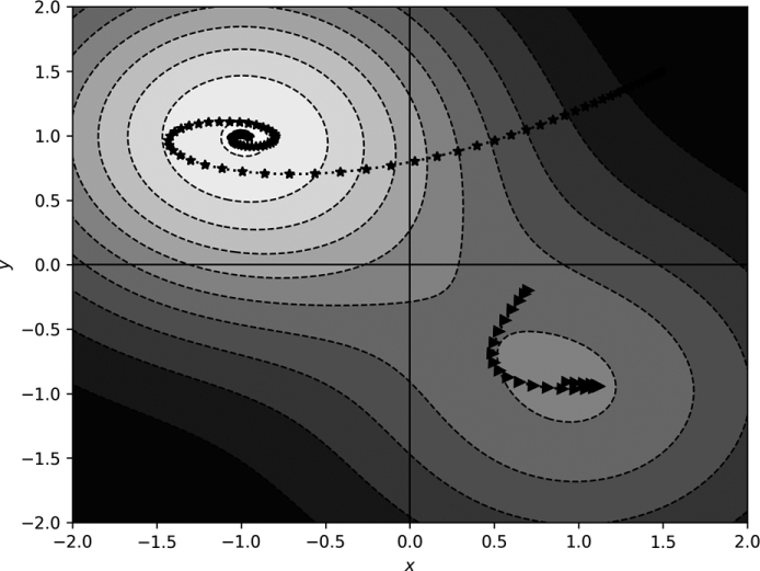
Figure 11-7: Gradient descent in two dimensions with momentum
Compare the paths in Figure 11-7 with those in Figure 11-5. Adding momentum has pushed the paths, so they tend to keep moving in the same direction. Notice how the path beginning at (1.5, 1.5) spirals toward the minimum, while the other path curves toward the shallower minimum, passes it, and backtracks toward it again.
The momentum term alters the dynamics of motion through the function space. However, it’s not immediately evident that momentum adds anything helpful. After all, the (1.5, 1.5) starting position using vanilla gradient descent moved directly to the minimum position without spiraling.
Let’s add momentum to our NN.py toolkit and see if it buys us anything when training real neural networks.
Training Models with Momentum
To support momentum in NN.py, we need to tweak the FullyConnectedLayer method in two places. First, as shown in Listing 11-4, we modify the constructor to allow a momentum keyword:
def __init__(self, input_size, output_size, momentum=0.0):
self.delta_w = np.zeros((input_size, output_size))
self.delta_b = np.zeros((1,output_size))
self.passes = 0
self.weights = np.random.rand(input_size, output_size) - 0.5
self.bias = np.random.rand(1, output_size) - 0.5
❶ self.vw = np.zeros((input_size, output_size))
self.vb = np.zeros((1, output_size))
self.momentum = momentum
Listing 11-4: Adding the momentum keyword
Here, we add a momentum keyword, with a default of zero, into the argument list. Then, we define initial velocities for the weights (vw) and biases (vb) ❶. These are matrices of the proper shape initialized to zero. We also keep the momentum argument for later use.
The second modification is to the step method, as Listing 11-5 shows:
def step(self, eta):
❶ self.vw = self.momentum * self.vw - eta * self.delta_w / self.passes
self.vb = self.momentum * self.vb - eta * self.delta_b / self.passes
❷ self.weights = self.weights + self.vw
self.bias = self.bias + self.vb
self.delta_w = np.zeros(self.weights.shape)
self.delta_b = np.zeros(self.bias.shape)
self.passes = 0
Listing 11-5: Updating the step to include momentum
We implement Equation 11.5, first for the weights ❶, then for the biases in the line after. We multiply the momentum (μ) by the previous velocity, then subtract the average error over the minibatch, multiplied by the learning rate. We then move the weights and biases by adding the velocity ❷. That’s all we need to do to incorporate momentum. Then, to use it, we add the momentum keyword to each fully connected layer when building the network, as shown in Listing 11-6:
net = Network()
net.add(FullyConnectedLayer(14*14, 100, momentum=0.9))
net.add(ActivationLayer())
net.add(FullyConnectedLayer(100, 50, momentum=0.9))
net.add(ActivationLayer())
net.add(FullyConnectedLayer(50, 10, momentum=0.9))
net.add(ActivationLayer())
Listing 11-6: Specifying momentum when building the network
Adding momentum per layer opens up the possibility of using layer-specific momentum values. While I’m unaware of any research doing so, it seems a fairly obvious thing to try, so by now, someone has likely experimented with it. For our purposes, we’ll set the momentum of all layers to 0.9 and move on.
How should we test our new momentum? We could use the MNIST dataset we used above, but it’s not a good candidate, because it’s too easy. Even a simple fully connected network achieves better than 97 percent accuracy. Therefore, we’ll replace the MNIST digits dataset with another, similar dataset that’s known to be more of a challenge: the Fashion-MNIST dataset. (See “Fashion-MNIST: A Novel Image Dataset for Benchmarking Machine Learning Algorithms” by Han Xiao et al., arXiv:1708.07747 [2017].)
The Fashion-MNIST dataset (FMNIST) is a drop-in replacement for the existing MNIST dataset. It contains images from 10 classes of clothing, all 28×28-pixel grayscale. For our purposes, we’ll do as we did for MNIST and reduce the 28×28-pixel images to 14 ×14 pixels. The images are in the dataset directory as NumPy arrays. Let’s train a model using them. The code for the model is similar to that of Listing 10-7, except in Listing 11-7 we replace the MNIST dataset with FMNIST:
x_train = np.load("fmnist_train_images_small.npy")/255
x_test = np.load("fmnist_test_images_small.npy")/255
y_train = np.load("fmnist_train_labels_vector.npy")
y_test = np.load("fmnist_test_labels.npy")
Listing 11-7: Loading the Fashion-MNIST dataset
We also include code to calculate the Matthews correlation coefficient (MCC) on the test data. We first encountered the MCC in Chapter 4, where we learned that it’s a better measure of a model’s performance than the accuracy is. The code to run is in fmnist.py. Taking around 18 minutes on an older Intel i5 box, one run of it produced
[[866 1 14 28 8 1 68 0 14 0]
[ 5 958 2 25 5 0 3 0 2 0]
[ 20 1 790 14 126 0 44 1 3 1]
[ 29 21 15 863 46 1 20 0 5 0]
[ 0 0 91 22 849 1 32 0 5 0]
[ 0 0 0 1 0 960 0 22 2 15]
[161 2 111 38 115 0 556 0 17 0]
[ 0 0 0 0 0 29 0 942 0 29]
[ 1 0 7 5 6 2 2 4 973 0]
[ 0 0 0 0 0 6 0 29 1 964]]
accuracy = 0.8721000
MCC = 0.8584048
The confusion matrix, still 10 × 10 because of the 10 classes in FMNIST, is quite noisy compared to the very clean confusion matrix we saw with MNIST proper. This is a challenging dataset for fully connected models. Recall that the MCC is a measure where the closer it is to one, the better the model.
The confusion matrix above is for a model trained without momentum. The learning rate was 1.0, and it was trained for 40,000 minibatches of 64 samples. What happens if we add momentum of 0.9 to each fully connected layer and reduce the learning rate to 0.2? When we add momentum, it makes sense to reduce the learning rate so we aren’t taking large steps compounded by the momentum already moving in a particular direction. Do explore what happens if you run fmnist.py with a learning rate of 0.2 and no momentum.
The version of the code with momentum is in fmnist_momentum.py. After about 20 minutes, one run of this code produced
[[766 5 14 61 2 1 143 0 8 0]
[ 1 958 2 30 3 0 6 0 0 0]
[ 12 0 794 16 98 0 80 0 0 0]
[ 8 11 13 917 21 0 27 0 3 0]
[ 0 0 84 44 798 0 71 0 3 0]
[ 0 0 0 1 0 938 0 31 1 29]
[ 76 2 87 56 60 0 714 0 5 0]
[ 0 0 0 0 0 11 0 963 0 26]
[ 1 1 6 8 5 1 10 4 964 0]
[ 0 0 0 0 0 6 0 33 0 961]]
accuracy = 0.8773000
MCC = 0.8638721
giving us a slightly higher MCC. Does that mean momentum helped? Maybe. As we well understand by now, training neural networks is a stochastic process. So, we can’t rely on results from a single training of the models. We need to train the models many times and perform statistical tests on the results. Excellent! This gives us a chance to put the hypothesis testing knowledge we gained in Chapter 4 to good use.
Instead of running fmnist.py and fmnist_momentum.py one time each, let’s run them 22 times each. This takes the better part of a day on my old Intel i5 system, but patience is a virtue. The net result is 22 MCC values for the model with momentum and 22 for the model without momentum. There’s nothing magical about 22 samples, but we intend to use the Mann-Whitney U test, and the rule of thumb for that test is to have at least 20 samples in each dataset.
Figure 11-8 displays histograms of the results.
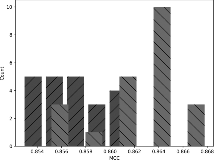
Figure 11-8: Histograms showing the distribution of MCC for models trained with momentum (light gray) and without (dark gray)
The darker gray bars are the no-momentum MCC values, and the lighter bars are those with momentum. Visually, the two are largely distinct from each other. The code producing Figure 11-8 is in the file fmnist_analyze.py. Do take a look at the code. It uses SciPy’s ttest_ind and mannwhitneyu along with the implementation we gave in Chapter 4 of Cohen’s d to calculate the effect size. The MCC values themselves are in the NumPy files listed in the code.
Along with the graph, fmnist_analyze.py produces the following output:
no momentum: 0.85778 +/- 0.00056
momentum : 0.86413 +/- 0.00075
t-test momentum vs no (t,p): (6.77398299, 0.00000003)
Mann-Whitney U : (41.00000000, 0.00000126)
Cohen's d : 2.04243
where the top two lines are the mean and the standard error of the mean. The t-test results are (t, p), the t-test statistic and associated p-value. Similarly, the Mann-Whitney U test results are (U, p), the U statistic and its p-value. Recall how the Mann-Whitney U test is a nonparametric test assuming nothing about the shape of the distribution of MCC values. The t-test assumes they are normally distributed. As we have only 22 samples each, we really can’t make any definitive statement about whether the results are normally distributed; the histograms don’t look much like Gaussian curves. That’s why we included the Mann-Whitney U test results.
A glance at the respective p-values tells us that the difference in means between the MCC values with and without momentum is highly statistically significant in favor of the with-momentum results. The t-value is positive, and the with-momentum result was the first argument. What of Cohen’s d-value? It’s a bit above 2.0, indicating a (very) large effect size.
Can we now say that momentum helps in this case? Probably. It produced better performing models given the hyperparameters we used. The stochastic nature of training neural networks makes it possible that we could tweak the hyperparameters of both models to eliminate the difference we see in the data we have. The architecture between the two is fixed, but nothing says the learning rate and minibatch size are optimized for either model.
A punctilious researcher would feel compelled to run an optimization process over the hyperparameters and, once satisfied that they’d found the very best model for both approaches, make a more definite statement after repeating the experiment. We, thankfully, are not punctilious researchers. Instead, we’ll use the evidence we have, along with the several decades of wisdom acquired by the world’s machine learning researchers regarding the utility of momentum in gradient descent, to state that, yes, momentum helps models learn, and you should use it in most cases.
However, the normality question is begging for further investigation. We are, after all, seeking to improve our mathematical and practical intuition regarding deep learning. Therefore, let’s train the with-momentum model for FMNIST, not 22 times but 100 times. As a concession, we’ll reduce the number of minibatches from 40,000 to 10,000. Still, expect to spend the better part of a day waiting for the program to finish. The code, which we won’t walk through here, is in fmnist_repeat.py.
Figure 11-9 presents a histogram of the results.
Clearly, this distribution does not look at all like a normal curve. The output of fmnist_repeat.py includes the result of SciPy’s normaltest function. This function performs a statistical test on a set of data under the null hypothesis that the data is normally distributed. Therefore, a p-value below, say, 0.05 or 0.01, indicates data that is not normally distributed. Our p-value is virtually zero.
What to make of Figure 11-9? First, as the results are certainly not normal, we aren’t justified in using a t-test. However, we also used the nonparametric Mann-Whitney U test and found highly statistically significant results, so our claims above are still valid. Second, the long tail of the distribution in Figure 11-9 is to the left. We might even make an argument that the result is possibly bimodal: that there are two peaks, one near 0.83 and the other, smaller one near an MCC of 0.75.
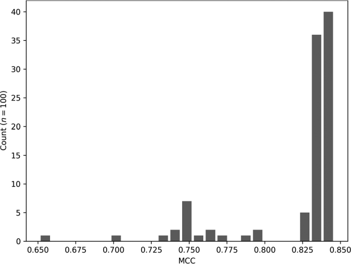
Figure 11-9: Distribution of MCC values for 100 trainings of the FMNIST model
Most models trained to a relatively consistent level of performance, with an MCC near 0.83. However, the long tail indicates that when the model wasn’t reasonably good, it was just plain horrid.
Intuitively, Figure 11-9 seems reasonable to me. We know stochastic gradient descent is susceptible to improper initialization, and our little toolkit is using old-school small random value initialization. It seems likely that we have an increased chance of starting at a poor location in the loss landscape and are doomed after that to poor performance.
What if the tail were on the right? What might that indicate? A long tail on the right would mean most model performance is mediocre to poor, but, on occasion, an especially “bright” model comes along. Such a scenario would mean that better models are out there, but that our training and/or initialization strategy isn’t particularly good at finding them. I think the tail on the left is preferable—most models find reasonably good local minima, so most trainings, unless horrid, end up in pretty much the same place in terms of performance.
Now, let’s examine a common variant of momentum, one that you’ll no doubt run across during your sojourn through deep learning.
Nesterov Momentum
Many deep learning toolkits include the option to use Nesterov momentum during gradient descent. Nesterov momentum is a modification of gradient descent widely used in the optimization community. The version typically implemented in deep learning updates standard momentum from
to

where we’re using gradient notation instead of partials of a loss function to indicate that the technique is general and applies to any function, f(x).
The difference between standard momentum and deep learning Nesterov momentum is subtle, just a term that’s added to the argument of the gradient. The idea is to use the existing momentum to calculate the gradient, not at the current position, x, but the position gradient descent would be at if it continued further using the current momentum, x + μ v. We then use the gradient’s value at that position to update the current position, as before.
The claim, well demonstrated for optimization in general, is that this tweak leads to faster convergence, meaning gradient descent will find the minimum in fewer steps. However, even though toolkits implement it, there is reason to believe the noise that stochastic gradient descent with minibatches introduces offsets the adjustment to the point where it’s unlikely Nesterov momentum is any more useful for training deep learning models than regular momentum. (For more on this, see the comment on page 292 of Deep Learning by Ian Goodfellow et al.)
However, the 2D example in this chapter uses the actual function to calculate gradients, so we might expect Nesterov momentum to be effective in that case. Let’s update the 2D example, minimizing the sum of two inverted Gaussians, and see if Nesterov momentum improves convergence, as claimed. The code we’ll run is in gd_nesterov.py and is virtually identical to the code in gd_momentum.py. Additionally, I tweaked both files a tiny bit to return the final position after gradient descent is complete. That way, we can see how close we are to the known minima.
Implementing Equation 11.6 is straightforward and affects only the velocity update, causing
vx = mu*vx - eta * dx(x,y)
vy = mu*vy - eta * dy(x,y)
to become
vx = mu * vx - eta * dx(x + mu * vx,y)
vy = mu * vy - eta * dy(x,y + mu * vy)
to add the momentum for each component, x and y. Everything else remains the same.
Figure 11-10 compares standard momentum (top, from Figure 11-7) and Nesterov momentum (bottom).
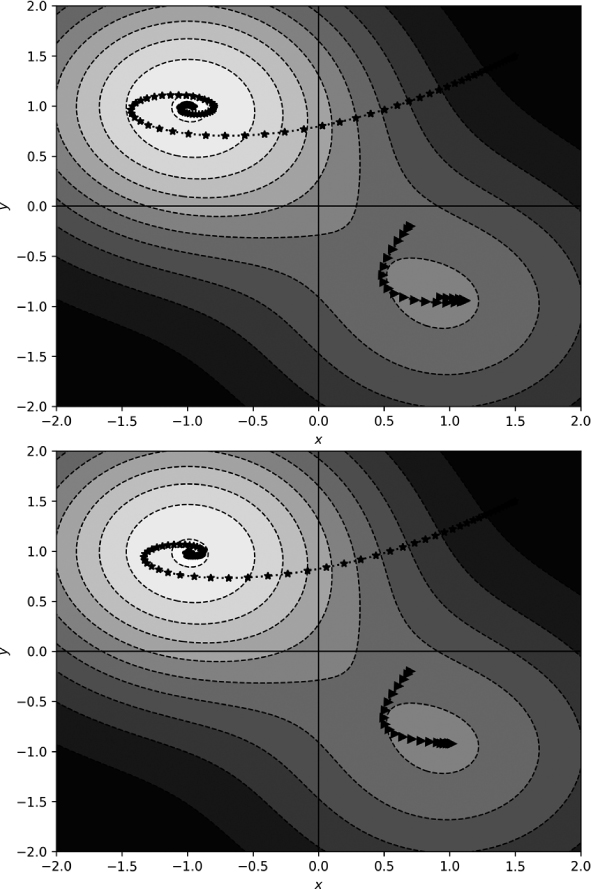
Figure 11-10: Standard momentum (top) and Nesterov momentum (bottom)
Visually, Nesterov momentum shows less of an overshoot, especially for the spiral marking the path beginning at (1.5, 1.5). What about the final location that each approach returns? We get Table 11-2.
Table 11-2: Final Location for Gradient Descent With and Without Nesterov Momentum
Initial point |
Standard |
Nesterov |
Minimum |
|---|---|---|---|
(1.5,1.5) |
(–0.9496, 0.9809) |
(–0.9718, 0.9813) |
(–1,1) |
(0.7,–0.2) |
(0.8807, –0.9063) |
(0.9128, –0.9181) |
(1,–1) |
The Nesterov momentum results are closer to the known minima than the standard momentum results after the same number of gradient descent steps.
Adaptive Gradient Descent
The gradient descent algorithm is almost trivial, which invites adaptation. In this section, we’ll walk through the math behind three variants of gradient descent popular with the deep learning community: RMSprop, Adagrad, and Adam. Of the three, Adam is the most popular by far, but the others are well worth understanding, as they build in succession leading up to Adam. All three of these algorithms adapt the learning rate on the fly in some manner.
RMSprop
Geoffrey Hinton introduced RMSprop, which stands for root mean square propagation, in his 2012 Coursera lecture series. Much like momentum (with which it can be combined), RMSprop is gradient descent that tracks the value of the gradient as it changes and uses that value to modify the step taken.
RMSprop uses a decay term, γ (gamma), to calculate a running average of the gradients as the algorithm progresses. In his lecture, Hinton uses γ = 0.9.
The gradient descent update becomes
First, we update m, the running average of the squares of the gradients, weighted by γ, the decay term. Next comes the velocity term, which is almost the same as in vanilla gradient descent, but we divide the learning rate by the running average’s square root, hence the RMS part of RMSprop. We then subtract the scaled velocity from the current position to take the step. We’re writing the step as an addition, similar to the momentum equations above (Equations 11.5 and 11.6); note the minus sign before the velocity update.
RMSprop works with momentum as well. For example, extending RMSprop with Nesterov momentum is straightforward:
with μ the momentum factor, as before.
It’s claimed that RMSprop is a robust classifier. We’ll see below how it fared on one test. We’re considering it an adaptive technique because the learning rate (η) is scaled by the square root of the running gradient mean; therefore, the effective learning rate is adjusted based on the history of the descent—it isn’t fixed once and for all.
RMSprop is often used in reinforcement learning, the branch of machine learning that attempts to learn how to act. For example, playing Atari video games uses reinforcement learning. RMSprop is believed to be robust when the optimization process is nonstationary, meaning the statistics change in time. Conversely, a stationary process is one where the statistics do not change in time. Training classifiers using supervised learning is stationary, as the training set is, typically, fixed and not changing, as should be the data fed to the classifier over time, though that is harder to enforce. In reinforcement learning, time is a factor, and the statistics of the dataset might change over time; therefore, reinforcement learning might involve nonstationary optimization.
Adagrad and Adadelta
Adagrad appeared in 2011 (see “Adaptive Subgradient Methods for Online Learning and Stochastic Optimization” by John Duchi et al., Journal of Machine Learning Research 12[7], [2011]). At first glance, it looks quite similar to RMSprop, though there are important differences.
We can write the basic update rule for Adagrad as
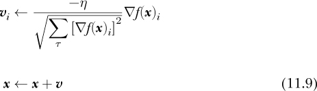
This requires some explanation.
First, notice the i subscript on the velocity update, both on the velocity, v, and the gradient, ▽f (x). Here, i refers to a component of the velocity, meaning the update must be applied per component. The top of Equation 11.9 repeats for all the components of the system. For a deep neural network, this means all the weights and biases.
Next, look at the sum in the denominator of the per-component velocity update. Here, τ (tau) is a counter over all the gradient steps taken during the optimization process, meaning for each component of the system, Adagrad tracks the sum of the square of the gradient calculated at each step. If we’re using Equation 11.9 for the 11th gradient descent step, then the sum in the denominator will have 11 terms, and so on. As before, η is a learning rate, which here is global to all components.
A variant of Adagrad is also in widespread use: Adadelta. (See “Adadelta: An Adaptive Learning Rate Method” by Matthew Zeiler, [2012].) Adadelta replaces the square root of the sum over all steps in the velocity update with a running average of the last few steps, much like the running average of RMSprop. Adadelta also replaces the manually selected global learning rate, η, with a running average of the previous few velocity updates. This eliminates the selection of an appropriate η but introduces a new parameter, γ, to set the window’s size, as was done for RMSprop. It’s likely that γ is less sensitive to the properties of the dataset than η is. Note how in the original Adadelta paper, γ is written as ρ (rho).
Adam
Kingma and Ba published Adam, from “adaptive moment estimation,” in 2015, and it has been cited over 66,000 times as of this writing. Adam uses the square of the gradient, as RMSprop and Adagrad do, but also tracks a momentum-like term. Let’s present the update equations and then walk through them:

The first two lines of Equation 11.10 define m and v as running averages of the first and second moments. The first moment is the mean; the second moment is akin to the variance, which is the second moment of the difference between a data point and the mean. Note the squaring of the gradient value in the definition of v. The running moments are weighted by two scalar parameters, β1 and β2.
The next two lines define ![]() and
and ![]() . These are bias correction terms to make m and v better estimates of the first and second moments. Here, t, an integer starting at zero, is the timestep.
. These are bias correction terms to make m and v better estimates of the first and second moments. Here, t, an integer starting at zero, is the timestep.
The actual step updates x by subtracting the bias-corrected first moment, ![]() , scaled by the ratio of the global learning rate, η, and the square root of the bias-corrected second moment,
, scaled by the ratio of the global learning rate, η, and the square root of the bias-corrected second moment, ![]() . The ∊ term is a constant to avoid division by zero.
. The ∊ term is a constant to avoid division by zero.
Equation 11.10 has four parameters, which seems excessive, but three of them are straightforward to set and are seldom changed. The original paper suggests β1 = 0.9, β2 = 0.999, and ∊ = 10−8. Therefore, as with vanilla gradient descent, the user is left to select η. For example, Keras defaults to η = 0.001, which works well in many cases.
The Kingma and Ba paper shows via experiment that Adam generally outperforms SGD with Nesterov momentum, RMSprop, Adagrad, and Adadelta. This is likely why Adam is currently the go-to optimizer for many deep learning tasks.
Some Thoughts About Optimizers
Which optimization algorithm to use and when depends on the dataset. As mentioned, Adam is currently favored for many tasks, though properly tuned SGD can be quite effective as well, and some swear by it. While it’s not possible to make a blanket statement about which is the best algorithm, for there is no such thing, we can conduct a little experiment and discuss the results.
This experiment, for which I’ll present only the results, trained a small convolutional neural network on MNIST using 16,384 random samples for the training set, a minibatch of 128, and 12 epochs. The results show the mean and standard error of the mean for five runs of each optimizer: SGD, RMSprop, Adagrad, and Adam. Of interest is the accuracy of the test set and the training clock time. I trained all models on the same machine, so relative timing is what we should look at. No GPU was used.
Figure 11-11 shows the overall test set accuracy (top) and the training time (bottom) by optimizer.
On average, SGD and RMSprop were about 0.5 percent less accurate than the other optimizers, with RMSprop varying widely but never matching Adagrad or Adam. Arguably, Adam performed the best in terms of accuracy. For training time, SGD was the fastest and Adam the slowest, as we might expect, given the multiple per-step calculations Adam performs relative to the simplicity of SGD. Overall, the results support the community’s intuition that Adam is a good optimizer.

Figure 11-11: MNIST model accuracy (top) and training time (bottom) by optimizer
Summary
This chapter presented gradient descent, working through the basic form, vanilla gradient descent, with 1D and 2D examples. We followed by introducing stochastic gradient descent and justified its use in deep learning.
We discussed momentum next, both standard and Nesterov. With standard momentum, we demonstrated that it does help in training deep models (well, relatively “deep”). We showed the effect of Nesterov momentum visually using a 2D example and discussed why Nesterov momentum and stochastic gradient descent might counteract each other.
The chapter concluded with a look at the gradient descent update equations for advanced algorithms, thereby illustrating how vanilla gradient descent invites modification. A simple experiment gave us insight into how the algorithms perform and appeared to justify the deep learning community’s belief in Adam’s general suitability over SGD.
And, with this chapter, our exploration of the mathematics of deep learning draws to a close. All that remains is a final appendix that points you to places where you can go to learn more.
Epilogue
As the great computer scientist Edsger W. Dijkstra said, “There should be no such thing as boring mathematics.” I sincerely hope you didn’t find this book boring. I’d hate to offend Dijkstra’s ghost. If you’re still reading at this point, I suspect you did find something of merit. Good! Thanks for sticking with it. Math should never be boring.
We’ve covered the basics of what you need to understand and work with deep learning. Don’t stop here, however: use the references in the Appendix and continue your mathematical explorations. You should never be satisfied with your knowledge base—always seek to broaden it.
If you have questions or comments, please do reach out to me at [email protected].