CHAPTER 5
Risk‐Neutral Valuation
While forward contracts separate the agreement date and the forward transaction date, they require both counterparties to abide by the terms of the forward contract, regardless of any profit or loss consideration. For example, the buyer in a forward contract has to buy the asset for the previously agreed upon price, even if the market price of the asset is below the contract price. An option contract, on the other hand, provides the right, but not the obligation, to transact an asset at some future date for predetermined terms. While the cash‐and‐carry argument allowed us to price a variety of forward contracts, the pricing of options requires more advanced techniques, and their pricing falls under the modern pricing paradigm of risk‐neutral valuation.
5.1 CONTINGENT CLAIMS
Option contracts are examples of contingent claims that allow the owner to transact at the option owner's sole discretion. We will focus on the economic value of the contract at transaction time and assume that an option owner will transact if and only if the economic value of the underlying transaction is positive.
The prime example of an option is a European‐style exercise option, which has a specified payoff at a specific exercise/expiration date ![]() in the future. For example, a European‐style call option,
in the future. For example, a European‐style call option, ![]() , with strike
, with strike ![]() on an asset
on an asset ![]() gives the owner the right—but not the obligation as opposed to a forward contract—to buy the asset for
gives the owner the right—but not the obligation as opposed to a forward contract—to buy the asset for ![]() at expiry
at expiry ![]() . At expiration, if the asset price is below the strike
. At expiration, if the asset price is below the strike ![]() , the option owner can buy the asset in the market for a lower price than
, the option owner can buy the asset in the market for a lower price than ![]() , and, hence, will not exercise the option and let it expire worthless. If the asset price is above
, and, hence, will not exercise the option and let it expire worthless. If the asset price is above ![]() , then the option owner can buy the asset for
, then the option owner can buy the asset for ![]() and sell it immediately in the market for
and sell it immediately in the market for ![]() for a profit of
for a profit of ![]() . The economic value of the option payoff is then
. The economic value of the option payoff is then

FIGURE 5.1 Economic value of European‐style call and put options at expiration with strike  .
.
Similarly, a put option with strike ![]() allows the owner to sell the asset at
allows the owner to sell the asset at ![]() at expiry and its economic value at expiration is
at expiry and its economic value at expiration is ![]() (see Figure 5.1).
(see Figure 5.1).
While the value of the contingent claim is known at expiration, the goal of contingent‐claim pricing is to determine its value prior to expiry. We will call the economic value of the option at expiry the option payoff, and focus on evaluating today's value of this future option payoff.
In 1973, the celebrated Black‐Scholes‐Merton (BSM) formula was derived to price European‐style call and put options [Black and Scholes, 1973]. While BSM methodology used advanced mathematical techniques to derive the formula, it was shown later by Cox‐Ross‐Rubinstein (CRR) [Cox et al., 1979] that the same formula can be obtained and understood using much simpler techniques. This new methodology goes under the name of risk‐neutral valuation and is the modern framework for contingent claim valuation. Its basic result is that any contingent claim's value is its expected discounted value of its cash flows in a risk‐neutral world [Harrison and Kreps, 1979; Harrison and Pliska, 1981].
5.2 BINOMIAL MODEL
Given today's ![]() price of an underlying asset
price of an underlying asset ![]() , consider a European‐style contingent claim
, consider a European‐style contingent claim ![]() with expiration
with expiration ![]() . Assume that the underlying asset has no cash flows over the period
. Assume that the underlying asset has no cash flows over the period ![]() , and let us consider the simplest case where the underlying asset at expiration can only take on two values
, and let us consider the simplest case where the underlying asset at expiration can only take on two values ![]() ,
, ![]() , as shown in Figure 5.2. Let
, as shown in Figure 5.2. Let ![]() and
and ![]() denote the corresponding then‐known values of the contingent claim in each state at expiration.
denote the corresponding then‐known values of the contingent claim in each state at expiration.

FIGURE 5.2 One‐step binomial model.
Our goal is to construct a replicating portfolio today so that the portfolio value at expiration (![]() ) replicates the value of the contingent claim. The fair price of the option today,
) replicates the value of the contingent claim. The fair price of the option today, ![]() , would be today's value of this replicating portfolio.
, would be today's value of this replicating portfolio.
Our portfolio consists of taking a position in the asset, ![]() units of it, with positive
units of it, with positive ![]() meaning buy and negative
meaning buy and negative ![]() meaning short, and entering into a loan or deposit at the prevalent continuously compounded risk‐free rate
meaning short, and entering into a loan or deposit at the prevalent continuously compounded risk‐free rate ![]() until
until ![]() . If
. If ![]() , we are borrowing money and if
, we are borrowing money and if ![]() we are lending. In either case, the value of the loan or deposit at expiration would be
we are lending. In either case, the value of the loan or deposit at expiration would be ![]() regardless of the state of the world.
regardless of the state of the world.
At ![]() , if we are in
, if we are in ![]() state of the world, we want this portfolio to be worth
state of the world, we want this portfolio to be worth ![]()
Similarly, if we are in ![]() state of the world, we want the portfolio to be worth
state of the world, we want the portfolio to be worth ![]()
We have two equations and two unknowns, ![]() . Solving for these, we get
. Solving for these, we get


Today's value of the contingent claim is

The seller of the option can charge ![]() , borrow or lend
, borrow or lend ![]() at interest rate of
at interest rate of ![]() , and use the proceeds to have
, and use the proceeds to have ![]() units of the asset priced at
units of the asset priced at ![]() . At expiration, in either state of the world,
. At expiration, in either state of the world, ![]() or
or ![]() , the value of her holdings (
, the value of her holdings (![]() units of the asset) exactly offsets her liabilities: loan or deposit amount plus interest,
units of the asset) exactly offsets her liabilities: loan or deposit amount plus interest, ![]() , and payment of the economic value of the option (
, and payment of the economic value of the option (![]() or
or ![]() ) to the option owner.
) to the option owner.
In Example 1, we are assuming fractional (50%) shares for exposition. For a more realistic example, assume that the call option allows one to buy 100 shares of the stock at the price ![]() per share. To replicate this option, one needs to buy 50 shares of the asset today at the price of $100 per share.
per share. To replicate this option, one needs to buy 50 shares of the asset today at the price of $100 per share.
The replication argument allows the buyer and the seller of the option to agree on the arbitrage‐free price of the option. The option buyer knows that by spending $3.44 per option, she can replicate the economic value of the option at expiration, and paying any amount less than $3.44 will result in a sure profit. In a competitive market with participants in search of sure profits, they will bid up the price of the option to the theoretical value until there are no sure profits left. Similarly, the option seller knows that by receiving $3.44 per option, she can own and, hence, deliver the economic value of the option at expiration, so any amount higher than that is a sure profit. In a competitive market, other participants will offer the option lower and lower until there are no sure profits left.
5.2.1 Probability‐Free Pricing
Note that in the above setup, we did not have to consider the probability of either state happening: as long as ![]() can happen and are the only two possibilities, we are golden!
can happen and are the only two possibilities, we are golden!
However, there are restrictions on the assumed future states. A bit of algebra allows us to rewrite the formula for ![]() as an expected value
as an expected value
where

and we recognize the ![]() term as the forward price
term as the forward price ![]() (see Figure 5.3).
(see Figure 5.3).
5.2.2 No Arbitrage
Lack of arbitrage is equivalent to ![]() being a probability
being a probability
which is equivalent to the following restriction on assumed states

FIGURE 5.3 Lack of arbitrage.
To see this, consider the case ![]() , which means that the forward is higher than either state in the future:
, which means that the forward is higher than either state in the future: ![]() . In this case, we can sell the asset forward for
. In this case, we can sell the asset forward for ![]() , and deliver it at
, and deliver it at ![]() by buying it at either
by buying it at either ![]() or
or ![]() . Regardless, we have made money with no risk.
. Regardless, we have made money with no risk.
Similarly, if ![]() , then
, then ![]() , and we can ensure a risk‐less profit by buying the asset forward for
, and we can ensure a risk‐less profit by buying the asset forward for ![]() , and selling it higher at expiration for
, and selling it higher at expiration for ![]() or
or ![]() .
.
Therefore, if there is no arbitrage in the above simple economy, ![]() can be considered as a probability, and today's value of the option is simply the expected discounted value of the option payoff under this probability per Formula 5.4.
can be considered as a probability, and today's value of the option is simply the expected discounted value of the option payoff under this probability per Formula 5.4.
5.2.3 Risk‐Neutrality
We obtained ![]() by constructing a portfolio that replicates the option payoff regardless of the probability of each state. We then showed that we can get the same value by taking the expected value under a probability
by constructing a portfolio that replicates the option payoff regardless of the probability of each state. We then showed that we can get the same value by taking the expected value under a probability ![]() . Other than a mathematical identity—
. Other than a mathematical identity—![]() is the probability that gets you the correct option value, as long as you know the option value—is there another way of interpreting
is the probability that gets you the correct option value, as long as you know the option value—is there another way of interpreting ![]() ? The answer is in the affirmative:
? The answer is in the affirmative: ![]() is the probability that a risk‐neutral investor would apply to the above setting. Consider two alternatives:
is the probability that a risk‐neutral investor would apply to the above setting. Consider two alternatives:
- Invest
 at the risk‐free rate
  , and receive
  at
at  .
. - Buy an asset at
 and either get
  or
or  at
at  .
.
For a risk‐neutral investor, these two investments would be equivalent if

which is identical to the expression in Formula 5.5. Therefore, rather than setting up a replicating portfolio and computing its value today, we can simply take the expected discounted value of the option payoff using risk‐neutral probabilities. Notice that Formula 5.6 can be rewritten as
relating the risk‐neutral probabilities directly to the assumed evolution of the asset. We can also rewrite Formula 5.4 as
with both of the above expectations using risk‐neutral probabilities.
5.3 FROM ONE TIME‐STEP TO TWO
The two‐state setup is obviously too simplistic. Assets can take a variety of values at expiration. However, using the above setup as a building block, we can arrive at more complex cases. The idea is to subdivide the time from now until expiration into multiple intervals, and for each state in each interval, generate two new arbitrage‐free (bracketing the forward) future states. With enough sub‐divisions, we can arrive at a richer and more real‐life terminal distribution for the asset.
Consider a two time‐step extension of the 1‐step binomial model shown in Figure 5.4. For each intermediate node ![]() at
at ![]() , we can use the 1‐step binomial model's Formulas, 5.8, and 5.9, to arrive at the risk‐neutral probabilities that would provide the same values for
, we can use the 1‐step binomial model's Formulas, 5.8, and 5.9, to arrive at the risk‐neutral probabilities that would provide the same values for ![]() as the replicating portfolios
as the replicating portfolios ![]() . Having computed
. Having computed ![]() , we can then use the 1‐step binomial model again to compute the risk‐neutral probabilities that would provide the same value as the replicating portfolio
, we can then use the 1‐step binomial model again to compute the risk‐neutral probabilities that would provide the same value as the replicating portfolio ![]() to compute
to compute ![]() .
.
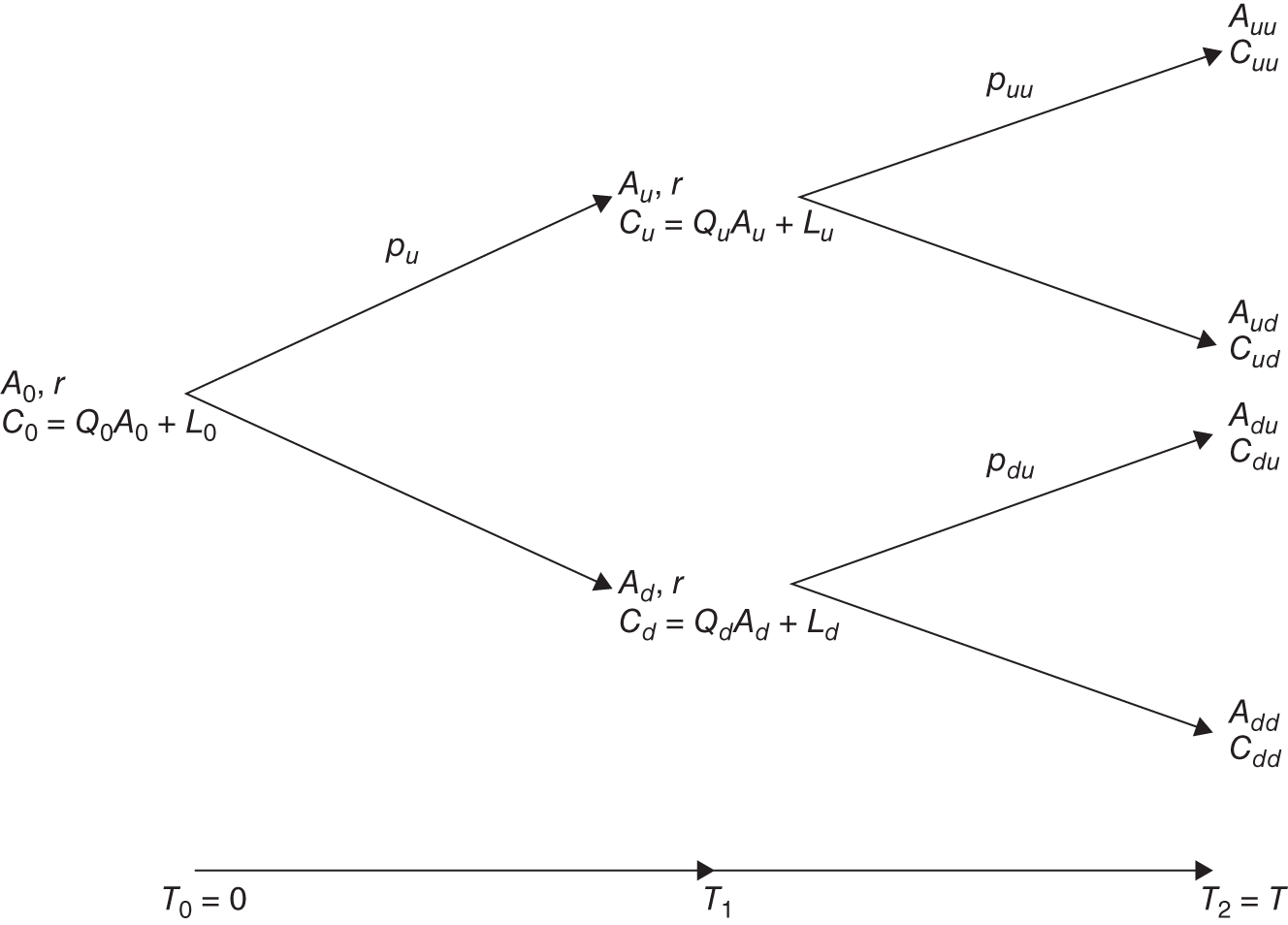
FIGURE 5.4 Two‐step binomial model.
5.3.1 Self‐Financing, Dynamic Hedging
As we subdivide the time to expiration into finer partitions, for the replication argument to hold, we have to ensure that the original portfolio is sufficient. We can change the composition of the portfolio, but cannot add new assets or unknown cash amounts. Therefore, at each interim state we can change the amount of the asset we hold by securing requisite funds at the prevailing financing rates. As we do this dynamic rebalancing (changing ![]() s), the value of the portfolio entering into each state must equal the value of the portfolio leaving the state, that is, the replicating portfolio should be self‐financing.
s), the value of the portfolio entering into each state must equal the value of the portfolio leaving the state, that is, the replicating portfolio should be self‐financing.
Consider the up state ![]() . As we enter it, we hold a portfolio that consists of
. As we enter it, we hold a portfolio that consists of ![]() units of the asset now worth
units of the asset now worth ![]() , and a loan of size
, and a loan of size ![]() plus its interest worth
plus its interest worth ![]() . Therefore, the value of the portfolio value is
. Therefore, the value of the portfolio value is
On the other hand, ![]() , since
, since ![]() is the required portfolio to replicate the option payoffs
is the required portfolio to replicate the option payoffs ![]() at the next time step
at the next time step ![]() . Therefore, we need to change our holding of the asset from
. Therefore, we need to change our holding of the asset from ![]() to
to ![]() only by changing the size of our loan from
only by changing the size of our loan from ![]() to
to ![]() , that is, the change in the underlying holding should only be financed by changing the loan size
, that is, the change in the underlying holding should only be financed by changing the loan size
ensuring that the portfolio is self‐financing. Similarly, in the down state ![]() , we have
, we have
5.3.2 Iterated Expectation
For the two time‐step model, at node ![]() , the risk‐neutral probability
, the risk‐neutral probability ![]() must satisfy
must satisfy

Having found ![]() , we can compute
, we can compute ![]()

Similarly, at node ![]() , the risk‐neutral probability
, the risk‐neutral probability ![]() must satisfy
must satisfy

to compute ![]()
The above formulas can be compactly written as conditional expectations conditioned on all information about an underlying asset up to ![]()

where both ![]() are random variables.
are random variables.
Having obtained ![]() , we can compute the risk‐neutral probability
, we can compute the risk‐neutral probability ![]() via
via

to get

and to compute ![]()
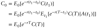
where we have used the law of iterated expectation: For any pair of random variables ![]()
where the outer expectation is taken relative to all possible outcomes of ![]() , see Appendix A.2.3. Combining Formulas 5.11 and 5.12, we have
, see Appendix A.2.3. Combining Formulas 5.11 and 5.12, we have
where the top equations in Formulas 5.10 and 5.13 characterize the risk‐neutral probabilities solely based on the assumed evolution of the underlying asset, while the bottom equations provide the valuation for any contingent claim.
5.4 RELATIVE PRICES
Formulas 5.10 and 5.13 can be generalized to ![]()

which can be written as
Let ![]() be the value of unit investment at a risk‐free rate, that is
be the value of unit investment at a risk‐free rate, that is ![]() equals the value of a money market account started with unit currency and continuously reinvested at the risk‐free rate.
equals the value of a money market account started with unit currency and continuously reinvested at the risk‐free rate. ![]() and
and ![]() . We have
. We have
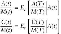
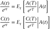
The first formula in 5.16 pins down the asset evolution in a risk‐neutral setting, while the second is the valuation formula for contingent claims. Note that we can always form a contingent claim whose payoff equals the value of the underlying, ![]() , therefore, the second formula already includes the first one and we can simply write
, therefore, the second formula already includes the first one and we can simply write

Probing Formula 5.17 further, it states that under risk‐neutral probabilities, relative prices for the asset and contingent claims on it relative to the money market account, ![]() , form a martingale: at any time
, form a martingale: at any time ![]() , the conditional expected future (
, the conditional expected future (![]() ) value is the
) value is the ![]() ‐value
‐value
or said differently, the conditional expected change between any two times is zero
A prime example of a martingale is the symmetric random walk (see Figure 5.6). At each time‐step, the expected value of the change is zero
Furthermore, no matter where we are in the future, say point ![]() or
or ![]() after four time‐steps, the expected value of the change from then on is still zero. This is a characterization of one's stake with payoff of
after four time‐steps, the expected value of the change from then on is still zero. This is a characterization of one's stake with payoff of ![]() based on the outcome of a fair (
based on the outcome of a fair (![]() ) coin. The expected amount of win or loss at each toss is 0 and the expected value of one's stake after any
) coin. The expected amount of win or loss at each toss is 0 and the expected value of one's stake after any ![]() tosses is the initial stake. The same holds for the future: if after
tosses is the initial stake. The same holds for the future: if after ![]() tosses we are at some level
tosses we are at some level ![]() , the expected value of the stake after another
, the expected value of the stake after another ![]() tosses is still the same level
tosses is still the same level ![]() .
.
5.4.1 Risk‐Neutral Valuation
We now have all the components of risk‐neutral valuation:
- Posit a random process for the evolution of the underlying assets.
- Adjust the process to ensure risk‐neutrality, equivalent to relative prices being martingales.
- The price of any contingent claim is the risk‐neutral expected discounted price of its cash flows.

FIGURE 5.6 A symmetric random walk is a martingale.
Note that ensuring risk‐neutrality is a condition on expectations that are composed of products of assumed states and their respective probabilities. This allows one to either fix the states and adjust the probabilities, or alternatively one can fix the probabilities and solve for the states. As long as expected relative prices satisfy Formula 5.17, we can use this probability‐adjusted or state‐adjusted evolution to price contingent claims.
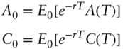
The risk‐neutral framework applies to non‐constant and random interest rates. In this case, the money market account's value becomes
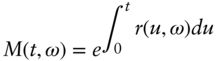
where ![]() denotes the randomness of future interest rates. This allows the risk‐neutral valuation framework to encompass interest rate derivatives (see Section 7.4.1).
denotes the randomness of future interest rates. This allows the risk‐neutral valuation framework to encompass interest rate derivatives (see Section 7.4.1).
5.4.2 Fundamental Theorems of Asset Pricing
The generalization of the above multi‐step model to an arbitrary number of assets and contingent claims based on them gives rise to the following Fundamental Theorems of Asset Pricing:
- For a given multi‐asset economy, lack of arbitrage is equivalent to the existence of probability distributions, which would make relative prices martingales. Each such probability distribution is called a risk‐neutral measure.
- A complete market is where every contingent claim can be replicated via a self‐financing trading strategy. A market is complete if and only if there exists a unique risk‐neutral measure.
The first condition is a generalization of the result that to preclude arbitrage, forward prices should be bracketed by assumed future states.
The second condition is the generalization of our ability to solve the replication equations, i.e., two equations and two unknowns. Had we assumed that starting from two assets—a bank loan and an asset—the number of future states in the next time‐step could be different than two, we would have had a different number of equations than unknowns, leading to generally either no solution or many solutions and, hence, a range of values for the contingent claim. In this case, the market would not be complete and contingent claims would not have a unique replicating portfolio or price.
REFERENCES
- Black, F. and Scholes, M. (1973). The pricing of options and corporate liabilities. Journal of Political Economy 81: 637–659.
- Cox, J.C., Ross, S.A., and Rubinstein, M. (1979). Option pricing: A simplified approach. Journal of Financial Economics 7: 229–263.
- German, H., El Karoui, N., and Rochet, J.C. (1995). Changes of numeraire, changes of probability measure, and option pricing. Journal of Applied Probability 32: 443–458.
- Harrison, J.M. and Kreps, D.M. (1979). Martingales and arbitrage in multi‐period securities markets. Journal of Economic Theory 20: 381–408.
- Harrison, J.M. and Pliska, S.R. (1981). Martingales and stochastic integrals in the theory of continuous trading. Stochastic Processes and Their Applications 11: 215–260.
EXERCISES
- Assume the risk‐free continuously compounded interest rate is 4% per annum. For an asset with today's price
 , you are told that its expected return is 10% per annum and that the asset in one year's time can be
  with probabilities
  . What is the expected value of the asset in one year in a risk‐neutral setting?
 - For each step of the risk‐neutral binomial model, what is the expected continuously compounded yield

- Let
 be the risk‐free continuously compounded rate and
  today's value of an asset. For a given horizon
  , assume the asset can take on two values
  with risk‐neutral probabilities of
  . Provide an expression for
  if
if  for a given volatility parameter
  .
. - In a 1‐step binomial model, compute the risk‐neutral probabilities for some
 when
when
- In the 1‐step binomial model shown in Figure 5.2, consider the portfolio consisting of one long position in the contingent claim and short

of the asset,
 .
.- Show that the portfolio has the same value at
 regardless of the terminal state
  , that is
  for a constant
  and the portfolio is risk‐less.
 - Using an arbitrage argument, show that today's value of the portfolio should be its discounted future value
and compute
 .
. - Show that the computed value of
 above is the same as Formula 5.3.
- Show that the portfolio has the same value at
- Using the same numerical values as in the 2‐period binomial model in Example 2
- Calculate today's price,
 , of a 6‐month European put option with strike
  .
. - Calculate today's value of a 6‐month forward contract with purchase price
 .
. - Verify that
 .
.
- Calculate today's price,
- Replication via Forward Contracts. In the 1‐step binomial model, replicate the option payoff at expiration via
 amount of a forward contract with delivery price of
  .
.
- Solve for


- Compute today's value of the above replicating forward contract:
 .
. - Is
 the same as Formula 5.3?
- Solve for
- Given two independent random variables

- Provide an expression for
 .
. - Evaluate the above when
 .
.
- Provide an expression for
- Let
 be independent and identically distributed random variables with
  , and let

Show that
 form a martingale
- For the random walk shown in Figure 5.6
- What is the expected movement during each period?
- What is the standard deviation of the movement during each period?
- What is the expected movement over
 time periods

- What is the standard deviation of the movement over
 time periods
