7.1 The ODE solvers for solving ordinary differential equations

ODE solvers are intended for first-order single or multiple ordinary differential equations that have the form:

$\frac{d{y}_1}{dt}=f_1\left(t,y_1,y_2,\dots ,y_n\right)$

$\frac{d{y}_2}{dt}=f_2\left(t,y_1,y_2,\dots ,y_n\right)$

…

$\frac{d{y}_n}{dt}=f_n\left(t,y_1,y_2,\dots ,y_n\right)$

where n is the number of first-order ODEs, y₁, y₂, . . ., y_n are the dependent variables, and t is the independent variable; the variable x can be used instead of t. High-order ODEs should be reduced to first order by creating a set of first-order equations. For example:

■ The equation
$\frac{d^{2}y}{d{t}^2}+0.5{\left(\frac{dy}{dt}\right)}^{2}y=sin\left(t\right)$
can be rewritten as two first-order equations
$\frac{d{y}_1}{dt}=y_2,\frac{d{y}_2}{dt}=-0.5y_2^2{y}_1+sin\left(t\right)$
In this case y₁(t) and y₂(t) values should be defined using the ODE solver.

■ The equation
$\frac{d^{3}y}{d{t}^3}+a\left[{\left(\frac{dy}{dt}\right)}^2+\frac{y}{t}\right]=sin\left(t\right)$
should be rewritten as three first-order ODEs:
$\frac{d{y}_1}{dt}=y_2,\frac{d{y}_2}{dt}=y_3,\frac{d{y}_3}{dt}=-a\left[y_2^2+\frac{y_1}{t}\right]+sin\left(t\right)$
In this case y₁(t), y₂(t), and y₃(t) values should be defined.

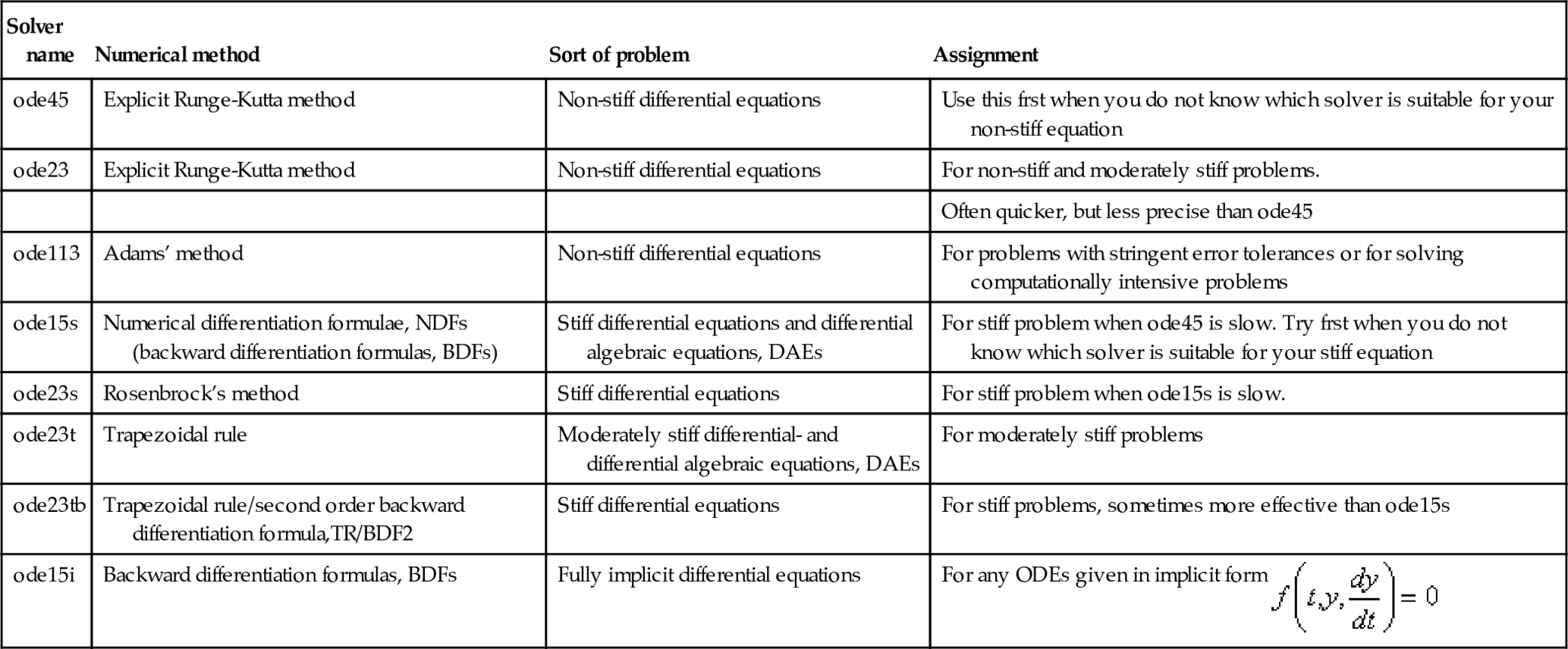
Unfortunately, there is no universal method for numerically solving any of the ODEs. Therefore, a number of solvers, realizing different methods, are used to solve an actual ODE. Table 7.1 lists the available solvers, the numerical method each solver uses, and the class of problem associated with each solver. These solvers are intended for so-called initial-value problems, IVP, when the differential equation is solved with any initial value of the function, e.g., y = 0 at t = 0 for the (dy / dt) = f(t, y) equation. An ODE solution with two boundary values specified at opposite ends of a range is called a boundary-value problem, BVP. In this chapter, we study IVP equations only; BVP equations are beyond the scope of this book.

Table 7.1

MATLAB® ODE solvers¹

Solver name	Numerical method	Sort of problem	Assignment
ode45	Explicit Runge-Kutta method	Non-stiff differential equations	Use this frst when you do not know which solver is suitable for your non-stiff equation
ode23	Explicit Runge-Kutta method	Non-stiff differential equations	For non-stiff and moderately stiff problems.
			Often quicker, but less precise than ode45
ode113	Adams’ method	Non-stiff differential equations	For problems with stringent error tolerances or for solving computationally intensive problems
ode15s	Numerical differentiation formulae, NDFs (backward differentiation formulas, BDFs)	Stiff differential equations and differential algebraic equations, DAEs	For stiff problem when ode45 is slow. Try frst when you do not know which solver is suitable for your stiff equation
ode23s	Rosenbrock’s method	Stiff differential equations	For stiff problem when ode15s is slow.
ode23t	Trapezoidal rule	Moderately stiff differential- and differential algebraic equations, DAEs	For moderately stiff problems
ode23tb	Trapezoidal rule/second order backward differentiation formula,TR/BDF2	Stiff differential equations	For stiff problems, sometimes more effective than ode15s
ode15i	Backward differentiation formulas, BDFs	Fully implicit differential equations	For any ODEs given in implicit form $f\left(t,y,\frac{dy}{dt}\right)=0$

7.2 Numerical methods and the ODE solvers

The main concept behind solving ODE equations is that the derivatives are replaced by finite differences according to the equation:

$\frac{dy}{dt}\to {\displaystyle \underset{\Delta t\to 0}{lim}}\frac{\Delta y}{\Delta t}=\frac{y_{i+1}-y_i}{t_{i+1}-t_i}$

which is apparently true for very small but finite (non-zero) distances between points; Δt and Δy are the argument and function differences and i is the point number in the [a,b]-range of the argument t. By giving the initial, first-point value y₀ at t₀ and calculating the value of ${\left.\frac{dy}{dt}\right|}_0=f\left(t_0,y_0\right)$, we determine the next y_1. Now by calculating ${\left.\frac{dy}{dt}\right|}_1=f\left(t_1,y_1\right)$ for the next argument, t₁, we determine y₂; repeating the process until final t all function values in the range are available. This approach, first realized by Euler, is used with improved and complex advanced numerical methods such as those of Runge-Kutta, Rosenbrock, Adams, etc.

ODE solvers can solve implicit non-stiff and stiff problems as well as fully explicit problems. There is no rigorous criterion for defining stiffness in the case of the two first categories of ODEs. Solving an equation that contains terms that lead to singularities (e.g., jumps in the function, holes, ruptures or others) results in a divergence in the numerical solution, even when using very small steps; thus, this type of ODE is referred to as stiff. In contrast to these equations, non-stiff ODEs are characterized by a stable convergence solution. Unfortunately, it is impossible to define a priori if the equation is stiff or not; therefore, it is impossible to determine in advance which ODE solver should be used. When solving an ODE that simulates a real technology or phenomenon we are prompted to select a specific ODE solver. For example, volatile processes, fast chemical reactions, explosions, etc, are described using stiff equations and thus stiff ODE solvers should be used (see Table 7.1). Sometimes, a ratio of the maximal to minimal coefficients of the ODE is used as a criterion of the stiffness; if this ratio is larger than 1000, the problem is categorized as stiff. This criterion is empirical and not always correct; consequently, in cases when the ODE type is not known a priori, it is recommended to use the ode45 solver first, and then the ode15s.

When an ODE is represented in the implicit form $f\left(\frac{dy}{dt},t,y\right)=0$ and cannot be transformed to the explicit form $\frac{dy}{dt}=f\left(t,y\right)$, the ode15i solver should be used. Implicit forms of ODEs are rarely found in the QA sciences and thus, they will not be discussed further.

7.3 The ODE solver command forms and steps for their solution

All ODE commands, with the exception of ode15i, take an identical form; the simplest record is:

[t,y]=ode. . .(@ode_fun,t_range,y0)

where

■ the ode. . . is one of the solver names, e.g., ode45 or ode15s; note, that ellipsis, . . ., should not be written in a real command as it signs the place for the solver number;

■ argument t is the output vector of t-points at which the y-values are calculated;

■ y is the output vector with the calculated function values that were calculated by the solver for the ODE, when more than one ODEs y is a matrix in which the first column is y₁ values, in the second y₂, etc.;

■ the @ode_fun is the function or function file name where differential equations should be written. The definition line of the function that contains the ODE should be
function dy=function_name(t,y)
In the lines below this function definition, the first-order differential equation/s should be written:
dy=[right side of the first ODE; right side of the second ODE; . . .];

■ t_range specifies the integration range, e.g. [1 14] defines a t-interval from 1 to 14; this vector can be written using more than two values when we want to display a solution at certain points in the range, e.g. [1:3:10 14] means that the results of the solution lie in the t-range of 1 . . . 14 and will be displayed at t-values of 1, 4, 7, 10 and 14; the values given in the t_range affect the output but not the step that ensures the tolerance, so that the resulting y-values are computed with default absolute tolerance 0.000001;

■ y0 is a vector with values of y-functions at initial t-points; in other words, this vector should contain the initial conditions, e.g. for a set of two first-order differential equations with initial function values y₁ = 0 and y₂ = 4, this vector is y0=[0 4]; vector y0 can also be given as a column, e.g., y0=[0;4]. Note: The ode. . . commands can be used without the output parameters t and y; in this case, a plot of the obtained y(t) solution appears after running the actual ode. . . .

Steps for solving an ODE

1. First, the equation should be presented in the form:

$\begin{array}{ll}\frac{dy}{dt}=f\left(t,y\right),\hfill & a\le t\le b\text{,}\hfill \end{array}$

with the initial condition

y=y₀ at t=t₀

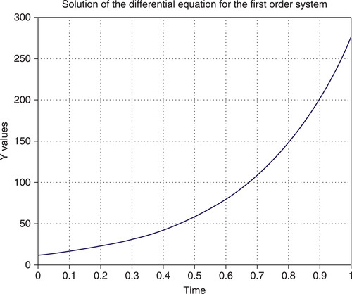
For this and the next steps we use a differential equation for a so-called first-order system, $b\frac{dy}{dt}+cy=0$. This equation describes many different phenomena: electrical RC circuits, e.g. for measuring a device, population dynamics, cooling of materials and liquids, and many other technological and physical processes; y in this equation is a dependent variable that denotes seeking a function at time t (independent variable); c and b are constants; for example, c = 1.1 and b = 0.35, the time range is 0 . . . 2 and initial value is y₀ = 12. The values are given in non-dimensional units, and in this case, the equation and its solution can be used for different real objects. For a numerical solution using one of the ODE solvers, the equation should be rewritten as:

$\frac{dy}{dt}=-\frac{c}{b}y$

2. In the second step, create the function files containing a use-defined function with a solving equation. The definition line of this function must include input arguments t and y and the output argument dy denoting the left-hand side of the ODE, dy/dt. In the next lines, write the ODE/s as a vector/s of right-hand parts of equation/s with the semicolon ( ; ) sign between them. Type the function file into the Editor Window and then save it with a name given in the definition line.

In our example we have one differential equation only and the function containing the differential equation is:

function dy=myODE(t,y)

dy=[-1.1/.35*y];

This function should be saved in m-file with the myODE name.

Note:

■ When the t- argument is absent in the right-hand part of the differential equation, the tilde (~) character can be written instead of this argument and the function definition line may appear as: function dy=myfODE(~,y)

■ In the case of a set of ODEs, the right-hand parts of this equation can also be written on separate lines, each in the dy vector, e.g., two ODEs

$\begin{array}{l}\frac{d{y}_1}{dt}=y_2\hfill \\ \frac{d{y}_2}{dt}=-0.2y_2+0.03y_1+cos\left(\omega t\right)\hfill \end{array}$

can be written as

dy=[y(2)

-0.2*y(2) + 0.03y(1)+cos(omega*t)]

instead of

dy=[y(2); -0.2*y(2)+0.03y(1)+cos(omega*t)].

3. In the final step, the stiffness of the ODE should be assumed together with the required numerical method of the solution, and then the corresponding ODE solver should be chosen from Table 7.1. For our example, when specific recommendations about appropriate methods are absent, the ode45 solver should be selected. The following command should be typed and entered in the Command Window:

$\begin{array}{ll}\gg \left[\mathrm{t},\mathrm{y}\right]=\mathrm{ode}15\mathrm{s}\left(@\mathrm{myODE},\left[0:.4:2\right],12\right)\hfill & \%\mathrm{t}=0\dots 1,\mathrm{step}.1;\hfill \\ \hfill & \%\mathrm{y}0=12\hfill \end{array}$

t =

0

0.4000

0.8000

1.2000

1.6000

2.0000

y =

12.0000

3.4135

0.9711

0.2763

0.0786

0.0224

The process starts with the initial value of y= 12 at t= 0; the final process time is t= 2, the time step for displaying the results was chosen at 0.4; thus, the vector of the time span, t_range, was input as 0:.4:2.

The given commands solve the equation and display two vectors with the resulting numbers. For plotting this solution, use the plot command, but seven t,y-points are not sufficient to generate a smoothed plot. To produce the plot, the t_range should be input with the start and final t-values. In this case, the default t-steps values will be automatically chosen and the resulting point number will be sufficient to generate a smoothed y(t) plot; the commands to be entered to achieve this are:

>> [t,y]=ode45(@myODE,[0 1], 12); % t=0 . . .1 with default step

>> plot(t,y)

>> xlabel('Time'),ylabel('Y values')

>> title('Solution of the differential equation for the first order system' )

>> grid

The generated plot is shown in Figure 7.1.

In the solution described above, part of the commands were written and saved in the myODE function file, and part of the commands – the ODE45, the plot, and plot formatting – were written in the Command Window. It is better to create a single program that includes all the commands; for this purpose, a function file should be written. For the example being studied, this file, named FirstOrderSystem, reads as follows:

function t_y=FirstOrderSystem(ts,tf,y0)

% Solution of the ODE for the first order system

% t – time; t_y – solution

% t_range=[ts tf];y0=12;

t_range=[ts,tf];

[t,y]=ode45(@myODE,t_range,y0);

plot(t,y)

xlabel('Time'),ylabel('Y values')

title('Solution of the differential equation for the first order system')

grid

t_y=[t y];

function dy=myODE(~,y)

dy=[-1.1/.35*y];

To run this file, input the following command from the Command Window:

>>t_y=FirstOrderSystem(0,2,12)

After entering the t and y values, they are displayed sequentially in two columns of 45 rows each (not listed here, for lack of space), and the graph (Figure 7.1), with the y as the function of time, is plotted.

7.4 Additional forms of the ODE solver commands

When the differential equation includes parameters such as b and c (as in the previously discussed example), which must be put into the function containing this equation, the more complicated ode . . . form is necessary:

[t,y]=ode. . .(@ode_fun,t_range,y0,[ ],arg_name1,arg_name2,. . .)

where [ ] denotes an empty vector. In general, this equation is the place for various options of integration and display control;² when this vector is empty, default values are used, which, in most cases, yield satisfactory solutions; these options are not used here. The names of the arguments that we intend to transmit to the ode_fun function are arg_name1, arg_name2,. . ..

The parameters named in the ode. . . command should also be written in the function containing ODE with these parameters.

In the previous example, the b and c coefficients in the FirstOrderSystem function can be introduced as arguments:

function t_y=FirstOrderSystem(b,c,ts,tf,y0)

% Solution of the ODE for the first order system

% t – time; t_y – solution

% t_range=[ts tf];y0=12;

t_range=[ts,tf];

[t,y]=ode45(@myODE,t_range,y0,[],b,c);

plot(t,y)

xlabel('Time'),ylabel('Y values')

title('Solution of the differential equation for the first order system')

grid

t_y=[t y];

function dy=myODE(~,y,b,c)

dy=[-1.1/.35*y];

To run this function, type and enter the following command in the Command Window:

>> t_y=FirstOrderSystem2(.35,1.1,0,2,12)

The results are identical to those described in Subsection 7.3.

The form having additional arguments is more advanced and has more versatility, e.g. the FirstOrderSystem function with arguments b and c can be used for problems described by the first-order system equation with the specific b and c coefficients.

In previously discussed forms, the ODE solver was used with the function written in a separate file or in a sub-function of the general function file. Another option is to introduce the ODE directly into the ode. . . solver command, in which case the general command form is

[t,y]=ode. . .(@(t,y) ode_fun(t,y, arg_name1,arg_name2,. . .), t_range,y0)

where @(t,y) ode_fun(t,y, arg_name1,arg_name2,. . .) is a function containing the right-hand part of the ODE with the additional arguments arg_name1,arg_name2,. . . that should be assigned beforehand; in this case, the ode_fun function can be written strictly within the ode. . . solver command.

This form permits the creation of a more compact program with lesser restrictions than in previous cases. This form of the command can be written and saved in a function file, a script file, or entered directly in the Command Window. To realize the latter possibility, write the following commands in the Command Window.

>>t_range=[0:.4:2]; b=0.35;c=1.1;

>>[t,y]=ode45(@(t,y) -c/b*y, t_range, 12)

t =

0

0.4000

0.8000

1.2000

1.6000

2.0000

y =

12.0000

3.4135

0.9711

0.2763

0.0786

0.0224

The results are displayed here at six time points t = 0, 0.4, 0.8, 1.2, 16, and 2.

7.5 Application examples

The programs below are mostly written in the form of a function, in which the first lines after the function description line are the help lines; these can contain a brief description and explanation of the input and output arguments of the function (see Chapter 4). In order to reduce the number of lines, the help line is written as a single line containing a command that should be input in the Command Window in order to run the function.

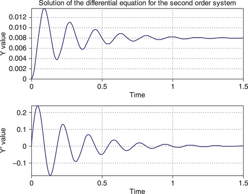
7.5.1 The second order dynamic system

Many technological systems used in quality control, for example metrological devices, can be described by the second-order dynamic system equation

$a\frac{d^{2}y}{d{t}^2}+b\frac{dy}{dt}+cy=F$

where y is the dependent variable, t is independent, e.g. time; and a, b, c, and F are constants having a different physical sense according to the actual problem.

Problem: Solve these equations and graph the results in two plots y(t) and $\frac{dy\left(t\right)}{dt}$ in the single Figure Window. Consider a = 1, b = 0.035, F = 9.8, the time interval 0 . . .1.5, and initial values y= 0 and $\frac{dy}{dt}=0$ at t = 0. Write a program as a function with a, b, c, F, ts (start time) and tf (finish time) as input values.

First represent the ODEs in the form suitable for the ODE solvers; to do this, rewrite the solving second order equation as a set of the two first order equations. Denote y= y₁ and $\frac{d{y}_1}{dt}=y_2$, and substitute this in the solving equation. The result provides the following system:

$\begin{array}{l}\frac{d{y}_1}{dt}=y_2\hfill \\ \frac{d{y}_2}{dt}=-\frac{1}{a}\left(b\frac{dy}{dt}+cy-F\right)\hfill \end{array}$

The second step is to select a suitable ODE solver. Since there is no specific information about the stiffness of the solving equations, the ode45 solver can be selected.

The final step is to create a function file with the ODE solver and sub-function containing the set of the ODEs to solve this problem. The Ch7_ApE1 function that solves the problem is:

function Ch7_ApE1(a,b,c,F,ts,tf,y0)

% to run: t_y=Ch7_ApE1(1,7,1225,9.8,0,1.5,[0;0])

t_range=[ts,tf];

[t,y]=ode45(@myODE_2,t_range,y0,[],a,b,c,F);

subplot(2,1,1)

plot(t,y(:,1))

xlabel('Time'),ylabel('Y value'),grid, axis tight

title('Solution of the differential equation for the second order system')

subplot(2,1,2)

plot(t,y(:,2))

xlabel('Time'),ylabel('Y value'),grid, axis tight

function dy=myODE_2(~,y,a,b,c,F)

dy=[y(2);-(b*y(2)+c*y(1)-F)/a];

This function is written as a function without output arguments. The input arguments – a, b, c and F – are the same as in the original equations; ts and tf are the start and the end times used by the ode45 in the t_range vector; y0 is the column vector with two initial y₁ and y₂ values. The set of solving equations is contained in the myODE_2 sub-function. The results are divided into two subplots using the subplot commands, and are shown using the plot commands, in which the first y-column represents the defined solution of the ODE, y(:,1), and the second is the derivative of the solution, y(:,2). To set better plot axes limits, the axis tight commands are used.

To run this function, type and enter the following command in the Command Window:

>> Ch7_ApE1(1,7,1225,9.8,0,1.5,[0;0])

After this the following graph with two sub-plots (Figure 7.2) is generated:

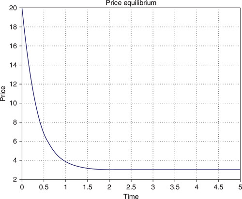
7.5.2 Equilibrium price and product quality enhancement

The equilibrium price is the price at which both the supply and the demand of an item are equal. For example, we calculate the equilibrium price when new technologies are used to enhance the production process in order to reduce the number of defective units. We use a model that includes the product price changes with the time, or, in other words, the derivative of the price by the time. The supply and demand equations in the model are

$\begin{array}{l}{Q}_d=a+bP+c\frac{dP}{dt}\hfill \\ Q_s=d-eP+g\frac{dP}{dt}\hfill \end{array}$

where P is the product price; $\frac{dP}{dt}$ is price change with time; a, b, c, d, e,and g are coefficients that should be known for actual product.

The demand Q_d should be equal to the supply Q_s:

$\frac{dP}{dt}=\frac{d-a-\left(e+b\right)P}{c-g}$

Problem: Solve this differential equation when a = 19, b = 1, c = 4, d = 28, e = 2 and g = 3, and the initial price is P₀ = 20. All the coefficients here are given in arbitrary units. Generate the price–time plot with the time values between 0 and 5.

First, represent this ODE in a form suitable for ODE solvers; for this, denote P = y and $\frac{dP}{dt}=\frac{dy}{dt}$. The resuit is the following ODE:

$\frac{dy}{dt}=\frac{d-a-\left(e+b\right)y}{c-g}$

The next step is to select a suitable ODE solver. As in the previous example, there is no specific information concerning the stiffness of the solving equation; thus, the ode45 solver can be selected.

The final step is to create a function file with the ODE solver and the sub-function containing the solving ODE. The Ch7_ApE2 function that solves the problem is:

function Ch7_ApE2(a,b,c,d,e,g,ts,tf,y0)

% To run:>>Ch7_ApE2(19,1,4,28,2,3,0,5,20)

t_range=[ts,tf];

[t,y]=ode45(@priceODE,t_range,y0,[],a,b,c,d,e,g);

plot(t,y)

xlabel('Time'),ylabel('Price')

title('Price equilibrium')

grid

function dy=priceODE (~,y,a,b,c,d,e,g)

dy=[(d-a-(e + b)*y)/(c-g)];

This function is written as a function without output arguments and the input arguments a, b, c, d, e and g are the same as in the original equation; ts and tf are the start and end times used by the ode45 in the t_range vector; y0 is the initial price of the product. The set of solving equations is contained in the sub-function priceODE.

To run this function, type and enter the following command in the Command Window:

Ch7_ApE2(19,1,4,28,2,3,0,5,20)

The following graph (Figure 7.3) is generated:

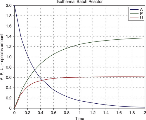
7.5.3 Batch reactor simulation

Various batch reactors are used in the biological and chemical industries to produce new products by means of the reactions of the initial reactants and catalysts. To optimize the process and to maintain quality, pre-simulation using a mathematical model is performed. Let us assume that the processes in a batch reactor are described by the following set of ordinary differential equations:

$\begin{array}{l}\frac{d\left[A\right]}{dt}=-k_1\left[A\right]-k_2{\left[A\right]}^2\hfill \\ \frac{d\left[P\right]}{dt}=k_1\left[A\right]\hfill \\ \frac{d\left[U\right]}{dt}=k_2{\left[A\right]}^2\hfill \end{array}$

where [A], [P], and [U] are the amounts of the species of the reactant A, the desired product P and the undesired product U respectively; the basic reactions that take place, A→ P and A + A→ U, have the respective k₁ and k₂ reaction rate constants.

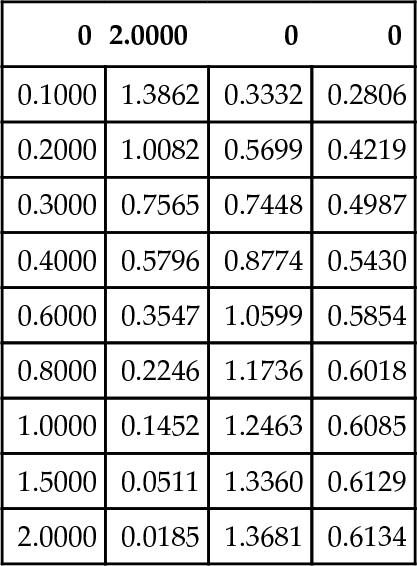
Problem: Solve these equations, display the results and plot the [A](t), [P] (t), and [U](t) curves in the time interval 0 . . . 2; the time values are equal to 0, 0.1, 0.2, 0.3, 0.4, 0.6, 0.8, 1, 1.5, and 2. The rate constants are k₁ = 2 for the first reaction and k₂ = 1 for the second. The initial amounts of the reagents are [A]₀ = 2 and [P]₀ = [U]₀ = 0. All the values are given here in arbitrary units and the time points are selected to obtain, display and generate as smooth a curve as possible using a small number of t-points.

First transmit the set of differential equations to the form required by the ODE solvers:

$\begin{array}{l}\frac{d{y}_1}{dt}=-k_1{y}_1-k_2{y}_1^2\hfill \\ \frac{d{y}_2}{dt}=k_1{y}_1\hfill \\ \frac{d{y}_3}{dt}=k_2{y}_1^2\hfill \end{array}$

Although no specific information is known about the stiffness of the ODE set, it is nevertheless known that chemical reactions can be very rapid; thus, it is reasonable to use the ode15s solver.

Finally, create the function file for this problem:

function t_A_D_U=Ch7_ApE3(k1,k2,ts,tf,A0,P0,U0)

% To run: >> t_A_P_U=Ch7_ApE3(2,1,0,2,2,0,0)

close all

t_range=[ts:.1:.4 0.6 0.8 1 1.5 tf];

[t,y]=ode15s(@BatchReactODEs, t_range,[A0,P0,U0],[],k1,k2);

plot(t,y)

xlabel('Time'),ylabel('A, P, U -species amount')

title('Isothermal Batch Reactor')

legend('A','P','U')

grid

t_A_P_U=[t,y];

function dy=BatchReactODEs (~,y,k1,k2)

dy=[-k1*y(1)-k2*y(1)^{^}2;k1*y(1);k2*y(1)^{^}2];

The input arguments k1, k2, and A0,P0,U0 respectively are the same as the k₁, k₂, and y₁, y₂ and y₃ values at t= 0 in the original set; the t_range is a two-element vector with a starting, ts, and final, tf, time value. The t_A_P_U output argument is a three-column matrix containing the time, reagent amount values, and the amounts of the desired and undesired products.

After running this function in the Command Window, the following results are displayed and plotted (Figure 7.4):

>>t_A_P_U=Ch7_ApE3 (2,1,0,2,2,0,0)

t_A_P_U =

0	2.0000	0	0
0.1000	1.3862	0.3332	0.2806
0.2000	1.0082	0.5699	0.4219
0.3000	0.7565	0.7448	0.4987
0.4000	0.5796	0.8774	0.5430
0.6000	0.3547	1.0599	0.5854
0.8000	0.2246	1.1736	0.6018
1.0000	0.1452	1.2463	0.6085
1.5000	0.0511	1.3360	0.6129
2.0000	0.0185	1.3681	0.6134

7.5.4 Grey model in predictive control charts

Grey models are used when there are few data and it is necessary to predict a system behavior on the data. In the case of the original data set x⁰(i), where i = 1, 2, . . ., n is the sample number or time in which the product was tested; the data transformed by the equation

$x^1\left(k\right)={\displaystyle \sum _{m=1}^k{x}^0\left(m\right)}$

can be described using the grey differential equation

$\frac{d{x}^1\left(k\right)}{dk}+a{x}^1\left(k\right)=u$

where the coefficients a and u can be obtained by the linear least-squares fit of the $\frac{d{x}^1}{dk}\left(x^1\right)$ data in which $\frac{d{x}^1}{dk}=\frac{\mathrm{diff}\left(x^1\right)}{\mathrm{diff}\left(k\right)}\equiv x^0\left(2:n\right)$ and x⁰ is taken beginning from the second value.

The predicted value of x⁰ for tested batch/time k + 1 is

$x^0\left(k+1\right)={\widehat{x}}^1\left(k+1\right)-{\widehat{x}}^1\left(k\right)$

where ${\widehat{x}}^1\left(k\right)$ and ${\widehat{x}}^1\left(k+1\right)$ are the values that are defined using the solution of the above ODE.

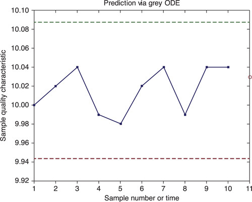
Problem: Average pin lengths in 10 sequentially tested samples were 10, 10.02, 10.06, 9.99, 9.98, 10.02, 10.04, 9.99, 10.04, and 10.04 mm; the upper and lower specification limits for pin length are 10.05 and 9.95 mm respectively. Using a grey model, predict the pin length value in the next test; use the polyfit command to define a and u in the grey ODE and then solve it using the ODE solver. Plot the control chart using the upper and lower control limits and the predicted value signed by the red o-marker.

To solve the problem the following steps should be taken:

■ Input the data as x_0 and transform them to x_1 with the cumsum command.

■ Calculate a and u using the polyfit command in which the first argument is – 0.5(x¹(i-1)+x¹(i)) and the second is $\frac{d{x}^1}{dk}=\frac{\mathrm{diff}\left(x^1\right)}{\mathrm{diff}\left(k\right)}\equiv x^0\left(2:n\right)$.

■ Solve the above ODE as $\frac{d{x}^1}{dk}=u-a{x}^1$ at sample numbers/times 1, 2,…, k, and k + 1, where k is the sample number/time; the beginning pin length value is the first pin length within the data.

■ Calculate the predicted value as $x^0\left(k+1\right)={\widehat{x}}^1\left(k+1\right)-{\widehat{x}}^1\left(k\right)$.

■ Plot the control chart with the predicted pin length value and the upper and lower control limit lines, defined as $\overline{x^0}\pm 3\sigma$ (where $\overline{x^0}$ is the average x⁰, and σ is the standard deviation of the x⁰).

To solve this problem, create the following function file:

function Ch7_ApE4(x_0)

% To run: Ch7_ApE4([10 10.02 10.04 9.99 9.98 10.02 10.04 9.99 %10.04 10.04])

close all

n=length(x_0);

x_1=cumsum(x_0);% transformed sequence

x_fit=-.5*(x_1(1:n-1) + x_1(2:n));

a_u=polyfit(x_fit,x_0(2:n),1)% a and u via fitting

[k,x_1_sol]=ode45(@mydif,1:n + 1,x_0(1),[],a_u);

x_0_predicted=x_1_sol(end)-x_1_sol(end-1);

average=mean(x_0);sigm=std(x_0);

UCL=average + 3*sigm;LCL=average-3*sigm;

x_CL=[1 k(end)];y_UCL=[UCL UCL];y_LCL = [LCL LCL]; % x and y-coord-s of CLs

plot(1:n,x_0,'.-',x_CL,y_UCL,'--',x_CL,y_LCL,'--',k(end),x_0_ predicted,'or')

xlabel('Sample number or time')

ylabel('Sample quality characteristic')

title('Prediction via grey ODE')

function dx=mydif(~,x,a_u)

dx=a_u(2)-a_u(1)*x;

After running this function with the command

>>Ch7_ApE4([10 10.02 10.04 9.99 9.98 10.02 10.04 9.99 10.04 10.04])

the graph appears on page 226 (Figure 7.5).

7.6 Questions for self-checking

1. When the stiffness of a differential equation is unknown, which ODE solvers are recommended to solve a problem: (a) ode23 first and then ode23t; (b) ode45 first and then ode15s; (c) ode15s first and then ode45; (d) ode113 and ode15s?

2. Which ODE solvers should be tried first for a non-stiff differential equation: (a) ode23tb, (b) ode15i, (c) ode45, (d) ode113?

3. To specify the interval for a differential equation solution, the t_range vector of an ODE solver should contain: (a) the single starting point value; (b) two values only – the starting and end points; (c) the starting point, the desired values within the interval, and the end points; (d) answers (b) and (c); (e) answers (a) and (b) are correct?

4. For solution of set of the two ODEs, the y0 vector in the ODE solver should include: (a) the y value for the first ODE only; (b) y values of each of the ODEs at initial point; (c) t values at starting points for each of the ODEs?

5. What occurs when the ODE solver command does not have output arguments: (a) an error message appears in the Command Window; (b) the Figure Window automatically appears with a plot of the obtained solution; (c) the obtained solution values automatically appear in the Command Window?

6. When a second order ODE must be solved, it should be: (a) written exactly as in a single second-order equation; (b) transferred to the set of the two first-order equations; (c) both answers (a) and (b) are possible?

7. In the [t,y]=ode45(@myODE,t_range,y0,[],a,b) command, the a and b input arguments are: (a) integration limits; (b) initial y values; (c) the names of the arguments that we intend to transmit to the myODE function?

8. The y' = f(y,t) solution with an ODE solver is: (a) the y(t) graph; (b) two vectors with t and y values; (c) a matrix with t and y values; (d) the y(t) graph and matrix of the t and y values?

9. To solve the y"-4y' + sin(x) = 0 equation using the ODE solvers: (a) rewrite the equation as y" = 4y'-sin(x); (b) leave the equation as written; (c) transform the equation to the set of the following equations $y_1^{\text{'}}=y_2$ and $y_2^{\text{'}}=y_2-sin\left(x\right)$?

7.7 Answers to selected questions

3. (d) answers (b) and (c) are correct.

5. (b) the Figure Window automatically appears with a plot of the obtained solution.

7. (c) the names of the arguments that we intend to transmit to the myODE function.

9. (c) transform the equation to the set of the following equations $y_1^{\text{'}}=y_2$ and $y_2^{\text{'}}=y_2-sin\left(x\right)$.