
Sensitivity analysis and big system engineering
Abstract
Sensitivity analysis is the science of determining the amount of variation a system has in response to specific range(s) of input. Sensitivity analysis has been applied to a wide range of analytic models and in particular to decompose the variance of the output. Sensitivity analysis is used for diagnostic modeling and in simulations, allowing system analysts to determine where to focus on system design to ensure robustness and accuracy across the range of inputs. In this chapter, we review the use of sensitivity analysis in ensemble selection and dimensionality reduction. Sensitivity analysis is then applied to ground truth and data pruning and used in specific applications, including the sensitivity in a linear set of equations, the sensitivity to added algorithms in a combinatorial or meta-algorithmic system, the sensitivity of an algorithm to its settings, and the path sensitivity to reach a given point in a distribution or path.
Keywords
Analytics; Data pruning; Dimensionality reduction; Ensembles; Ground truthing; Path; Sensitivity; Sensitivity analysis
Beauty of whatever kind, in its supreme development, invariably excites the sensitive soul to tears
Edgar Allan Poe (1846)
Manhood coerced into sensitivity is no manhood at all
Camille Paglia (1992)
5.1 Introduction
If you’ve made it this far and have been reading from the beginning, there is some good news. You’ve now covered enough to be confident, conversant, and even congruent when speaking to other analytic experts. The first four chapters were, in effect, the first half of the book and were intended to get the fundamentals of analytics across, albeit hopefully in a novel and more expansive manner than do comparative analytics texts.
The “second half” of this book focuses on incorporating important system level and/or novel approaches to the field of analytics. In so doing, meta-analytic systems are created. Another key focus in this chapter and Chapters 6–14 is their applications. We begin this half of the book with a consideration of how sensitivity analysis approaches can be employed for analytics. Building on two patterns for incorporating sensitivity analysis techniques, we then extend them to a number of important areas in meta-analytics; specifically, settings for individual algorithms and for hybrid systems of multiple algorithms. In line with Edgar Allan Poe, we are hoping the beauty of hybrid systems will not only move the sensitive soul to tears but also move the system architect to consider employing sensitivity techniques more robustly in their analysis. In line with Camille Paglia, we feel that the system designer need not be coerced into using sensitivity analysis; however, it probably wouldn’t hurt to appropriately justify it. As far as building analytics into the system from the ground up, then, “sensitivity analysis is considered … as a prerequisite for model building in any setting, be it diagnostic or prognostic, and in any field where models are used” [Salt04]. In Ref. [Salt04], they show that sensitivity analysis can and should be applied to a wide variety of analytic models and specifically to decomposing the variance of the output, in diagnostic modeling and in simulations.
In Chapter 4, we mentioned that sensitivity analysis is an underappreciated part of any analytics project. Sensitivity analysis can be applied directly to any of the “variables” in a system design, allowing a multilayered approach to assessing the robustness of a system and avoiding such “overtraining” traps as k-fold cross validation, which is effectively testing on the training data. In k-fold validation, the training set is often 90% of the available data for training and testing (k = 10), and the testing results are reported on 10% of the data at a time. Unless the training and testing data are highly uncorrelated—and even if they were, why would they be for a majority of the k = 10-folds?—this is effectively reporting testing results on training data (see Sections 1.10 and 1.11 for more on why this is not a good strategy).
This is the stick, but there is also a carrot: sensitivity analysis provides significant positive advantages. Sensitivity analysis is one of the best ways to determine how well a system comes together as a compound of its modules, by affording a mean of assessing the interfaces between components of a modular, large-scale system. In Chapter 4, we introduced the sensitivity-driven ensemble selection pattern, recapitulated here in light of the sensitivity:
- 1. First and foremost, sensitivity analysis is an assessment of the partial derivatives of the factors in the region of interest, that is,
 , or the relative magnitude of the partial derivative compared with the norm of the dependent variable in a region. After computing these, we rank the factors in the system based on their relative magnitudes. Dividing the partial derivative by the norm of the variable removes the need to normalize each variable in the region.
 - 2. Next, we determine the appropriate coefficients for the behavior of these factors in the region of interest. This means that we can weight each of the values by their contribution to error. This can be done by separately considering each factor as outlined in Section 1.11.
- 3. We can then multiply the outputs of (1) and (2) to get a weighted significance coefficient for each factor, implying this is the relative contribution of the factor to the overall (measured) system behavior.
- 4. Create a pool of algorithms for the ensemble with the overall coefficient for the algorithms proportional to the relatively weighted significance coefficient of each factor.
- 5. Deploy the ensemble and perform ensemble operations (boosting, bagging, etc.). In this way, the sensitivity-driven ensemble selection pattern proceeds with traditional ensemble techniques once the factors are identified, ranked, and relatively weighted.
A second sensitivity analysis pattern introduced in Chapter 4 was the sensitivity-driven dimensionality reduction pattern. Here, the relative sensitivity of each feature, y, to variation in the input, as above given by ![]() , is evaluated first. Other means of assessing the relative sensitivity are to use the magnitude of the range of y, or the standard deviation of y, rather than the norm ‖y‖. As mentioned previously, simultaneously employing the norm of y, the range of y, and the standard deviation of y and then combining the results using weighted voting are another way of adding potential robustness to the solution. However weighted, the features are then ranked in order, and we can remove the lowest-weighted features in order up to 5%, 10%, 20%, etc. of the overall sum of
, is evaluated first. Other means of assessing the relative sensitivity are to use the magnitude of the range of y, or the standard deviation of y, rather than the norm ‖y‖. As mentioned previously, simultaneously employing the norm of y, the range of y, and the standard deviation of y and then combining the results using weighted voting are another way of adding potential robustness to the solution. However weighted, the features are then ranked in order, and we can remove the lowest-weighted features in order up to 5%, 10%, 20%, etc. of the overall sum of ![]() over all y. This last filtering step allows us to remove any irrelevant attempts to add robustness, anyway. Thus, the combination of using a large array of features and then filtering is a useful design approach, in general.
over all y. This last filtering step allows us to remove any irrelevant attempts to add robustness, anyway. Thus, the combination of using a large array of features and then filtering is a useful design approach, in general.
In Chapter 3, we noted that sensitivity analysis typically focuses on a matrix of partial derivatives and/or conditional partial derivatives. We defined the “sensitivity” as the response of a system to an instantaneous change in a relevant part of its input. In particular, the sensitivity analysis of any model for the data is essential in modern system design (and should not be omitted). Suppose we have two models for fitting a set of data and their residual signals (the behavior of the data after subtracting out the model) are effectively equivalent. The two models are
Quick inspection shows that both models have the points (0.0, 1.23) and (1.0, 0.0) in common.
For sensitivity analysis, we find the partial derivatives (slopes) of these two simple models:
We see that Model A has a slope of 0 when x = 0.369 and Model B has a slope of 0 when x = 0.583. In general, though, we use a hybrid model, using Model A when
This becomes three equations, based on the ranges in x:
Rearranged, each of Eqs. (5.6), (5.7), and (5.8) becomes Eq. (5.9):
So, we use Model A whenever x < 0.944 and Model B whenever x > 0.944. As mentioned with a different example in Chapter 3, this provides us with a means to select multiple models for a domain. We can modify the coefficients of models so that there is smoothness (continuity) at the subdomain boundaries if desired. For example, we see that Model A has the value y = 0.316 when x = 0.944 and Model B has the value y =− 0.325 when x = 0.944, and so, switching from Model A to Model B at x = 0.944 would result in a large discontinuity at x = 0.944. Therefore, we may provide some moving average of the two models, ending at x = 1.0 where they are equal and, due to symmetry, starting the same distance in front of x = 0.944 (i.e., at x = 0.888). This is a totally acceptable strategy, called “blending,” and it reminds us that the goal to keep the sensitivity of the models to a minimum is only one aspect of the overall model. For example, if Eqs. (5.1) and (5.2) describe the cost of the system, we would be more concerned with accuracy than sensitivity per se.
5.2 Sensitivity analysis of the data set itself
In Section 3.4, the aging of data and statistical approaches to this important topic were overviewed. In this section, we address additional approaches to monitoring, augmenting, pruning, and otherwise maintaining throughout its life cycle the data that we use to define the model and its settings. We start off with a discussion of performing sensitivity analysis on the critical points for a classification feature selection procedure.
In Section 1.10, the concept of “critical points” between the means of two populations to be compared (for categorization, labeling, classification, and the like) was introduced. In that section, we simply rank ordered the means of the distributions and then computed the critical points to be between the consecutive means at the point that is the same number of standard deviations (usually a different value for each of the two populations) from the pair of means. If all populations have the same variance, then the critical points are simply the midpoints between the means. If there are N populations, this method defines N − 1 critical points. This approach, however, is readily generalized to cover any additional comparisons. If, for example, critical points are defined between a population and the two closest populations to either side of it in ranked order, then there are N − 1 critical points for the nearest neighbors and an additional N − 2 critical points for the second-nearest neighbors. In the extreme, where critical points of all possible lengths up to N − 1 are computed, there are a total of N(N − 1)/2 critical points, or ½(N2 − N) critical points. This is Order(N2) instead of the original Order(N).
So, in general, how do we decide how many critical points to define? One quantitative means of determining how many neighbors in each direction to compute critical points for is determinable by the ratio of the range of a single population to that of the set of all populations. Suppose that we have the following eight classes of training data, here defined by their means and standard deviations:
- 1. 45.7 ± 5.4
- 2. 56.8 ± 11.6
- 3. 65.4 ± 9.9
- 4. 66.9 ± 8.4
- 5. 72.7 ± 11.1
- 6. 73.4 ± 8.8
- 7. 81.6 ± 7.7
- 8. 83.2 ± 5.6
We see from this that the geometric mean of the standard deviation is the eighth root of the product (5.4 × 11.6 × 9.9 × 8.4 × 11.1 × 8.8 × 7.7 × 5.6) = 8.2. The samples themselves span the range 40.3–89.3 (the total range being 89.3 − 40.3 = 49.0) for mean ± standard deviation (note that the upper end is set by population 7 and not population 8, even though population 8 has a higher mean). The ratio is thus 8.2/49.0 = 0.167, and so, the range of all the populations is roughly six times that of a single population. Note that we could have just as simply made this the ratio of 1.96 standard deviations (alpha = 0.05), and the ratio would have been substantially different, that is, 16.1/(96.7 − 34.1)=0.257. Here, the range of all populations is roughly four times that of a single population. In general, then, we set the number of neighbors for which to compute critical points based on the alpha level and the following algorithm:
- 1. Find the upper level of the combined set of populations as the maximum value of the (population mean)+ nalpha ×(population standard deviation) across all populations, where nalpha is the number of standard deviations from the mean to obtain the desired alpha level of confidence in the mean, and this is 1.645 for alpha = 0.10, 1.96 for alpha = 0.05, 2.33 for alpha = 0.02, and 2.58 for alpha = 0.01 (two-tailed test). This is designated PopulationUPPER.
- 2. Find the lower level of the combined set of populations as the minimum value of the (population mean)− nalpha ×(population standard deviation) across all populations, where nalpha is the number of standard deviations from the mean to obtain the desired alpha level of confidence in the mean, and this is 1.645 for alpha = 0.10, 1.96 for alpha = 0.05, 2.33 for alpha = 0.02, and 2.58 for alpha = 0.01 (two-tailed test). This is designated PopulationLOWER.
- 3. Find the range of the overall set of populations = PopulationUPPER − PopulationLOWER.
- 4. Find the geometric mean of the range of the individual classes using the same probability alpha. This is simply nalpha multiplied by the NClasses-root of the product of all the class standard deviations. The value NClasses is the number of classes. For example, if nalpha is 8, as in our example, then it is the eighth root of the product. This is the geometric mean of the standard deviation of the classes, or GM(σClasses).
- 5. Find the mean range of the classes = 2⁎GM(σClasses).
- 6. Calculate the mean overlap ratio = MOR =(PopulationUPPER − PopulationLOWER)/2⁎GM(σClasses).
- 7. Set the number of neighbors to either side as NClasses/MOR. Round up to the nearest integer.
In the example given, MOR is the inverse of the 0.257 value computed for alpha = 0.05. Thus, MOR = 3.89, and the ratio of 8/3.89 = 2.06. We could round this up to three, in which case we define 7 + 6 + 5 = 18 critical points. However, using 2 instead of 3 neighbors, we have 7 + 6 = 13 critical points, which would probably work just as well. The main utility of the critical points, of course, is to comparatively assess features, and so, we can also adjust the number of nearest neighbors based on the size of the data set, the absolute number of classes, and the percentage of overlap between classes. Regardless, the seven-step algorithm given here will work well. We now turn our attention to other aspects of data set sensitivity analysis.
Characterizing the critical points gives us some preliminary insight into the nature of the ground truth, or training data, at hand. One aspect of meta-analytics is to go beyond the normal treatment of ground truth associated with regular analytics. The cumulative data set should be used to determine if data should be retired (age-based pruning), augmented (underrepresentation imputation of ground truth), or destabilized. Age-based pruning was covered in Section 3.4. Augmentation is simple enough. Underrepresented clusters, categories, or classes of data can have additional samples added directly (through the targeted collection of more samples) or indirectly (through simulation). Destabilization, however, merits a slightly deeper discussion.
Why do we want to “destabilize” data in the first place? Isn’t stability good? Not when the rest of the world is unstable. In data science as in politics, it is often risky and even ill-advised to be stable when all of your peers are unstable. Making sure that each subgroup of data has similar overall variability ensures similar robustness and “educational opportunity.” Often, stability in data sets is the data science equivalent of “teaching to the exams” in human education: the process of reducing the gamut of input, intentionally or unintentionally, generally makes the student or system less robust to new input [Kohn00]. Destabilization then is data “open-mindedness.”
Destabilization can legitimately be performed in several situations, including (a) when one set of ground truth has statistically significantly different entropy than the other sets, (b) when one set of ground truth is more or less qualitative/quantitative than the other sets, and (c) when one set of ground truth is created by different means than the other sets. A fourth, slightly different form of destabilization is (d) when the grouped behavior of the data is too similar by analytic evaluation. We address each of these in order.
One form of stabilization, (a) above, is also one of the easiest to discover, if you are looking. Data sets differing in entropy are likely examples of “selective oversampling,” wherein specific subgroups within a larger class are overrepresented. In many cases, such overrepresentation is all but inevitable, unless the experimentalist has an unlimited budget. Admittedly, in many of the examples in this book, data “stabilization” occurs, simply because I have access to a limited number/variety of sensing, recording, or other analysis equipment—not to mention conscious and/or subconscious bias to collect data suitable to illustrate the point(s) I intend to make in a given section of the text. Any time there is a bias, spoken or unspoken, in how data are captured, there is a risk of data stabilization. This occurs when one device is the adopted norm, due to ubiquity, cost, standards of practice, etc. It can also occur when the population available is not representative; for example, differences in ancestry vary greatly in comparing on campus to off campus, urban to suburban to rural, etc. Finally, it can occur due to differences in “setting bias” wherein one photographer prefers a different f-stop (aperture), shutter speed, ISO, focal length, and the like, and this set is different from that preferred by another photographer. This may lead to subtle differences in the data sets that are exposed once analytics are generated. To “destabilize” such data, we need to define a measure of entropy that partitions (or “discretizes”) one or more feature ranges and allows for a statistical comparison among the clusters, categories, or classes. In the case of a setting, the “bins” that are used to compute the individual probabilities from which the entropy (please see Eqs. (1.14) and (1.15) in Section 1.8.1) is computed may be derived directly from the menu options (e.g., only a discrete set of f-stops, shutter speeds, etc. are available). For other features, a reasonable histogram that partitions the space “fairly” should suffice.
The second type of destabilization occurs when the ground truth sets differ in their qualitative and/or quantitative nature. Using the example of camera settings, one camera may have only discrete settings, and another may have an analog dial that allows a continuum of settings. Another, say less expensive camera, may have a lot less f-stops altogether. It is not immediately clear how to impute values between discrete settings to have the same variety of behavior as those coming from a continuum. One means of destabilizing data coming from a less diverse environment is to add noise stochastically to match the spread of the more diverse environment. For example, a discrete setting can be treated as the mean of a distribution and a distribution fitted to it so that it covers the range between its two nearest critical points with the same amount of variance as in the other group taken from a continuum. This is another use of the critical points described earlier in this section.
A third setting for destabilization is when one set of ground truth (whether for training, validation, and/or testing) is created by a different process than the other sets. This can result in data artifacts that are indistinguishable from actual differences between groups but may change the nature of the differences and so remain hidden—unless the analytic expert is aware of the context (or metadata) for the data collection. Often, this form of stability occurs through imbalances in data collection, using referred to as inequalities of scale. These inequalities can include time, time of day, location, and demographic differences that may be compounded across groups. They may even be hidden by statistical tests. For example, features 1 and 2 for groups A and B may have had statistically nonsignificant differences for location, but when an ANOVA (analysis of variance) is performed, we see a statistically significant difference in comparing feature 2 for group B to feature 1 for group A. This interaction may strongly affect any group-to-group differences later reported. For this reason, ANOVA should be used for any multifactor feature set, if possible. When there are known to be inequalities of scale in comparing two or more data sets, data deletion, data augmentation, or data imputation should be considered. The latter can be performed as described above using the critical points between data groups.
A fourth form of destabilization is applicable when all groups have highly correlated analytic evaluation behavior. Functional outputs such as accuracy, cost, robustness, and other system behavior can be plotted against the amount of data used or the percentage of data used from the ground truth set. The different groups are then assessed based on the nature of these data graphs (or other visualizations). These assessments can be based on relative behavior of the different groups or on their pruning behavior (i.e., when removing the same percent of oldest, most suspect, lowest confidence, etc. training data) data. Sensitivity to pruning data may undercover some patterns in the data over time (e.g., unreported imputation and attempts to obscure highly correlated data)
5.3 Sensitivity analysis of the solution model
Solution models are broader than data models. Solution models generally describe the manner in which an input is converted into an output. The ratio of output to input is the transfer function, and it is often modeled as the ratio of two polynomials, which provides both convenience and generalizability (not to mention ease of building individual modules). We describe the system behavior as
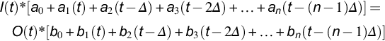
In Eq. (5.10), sensitivity analysis is rather straightforward. Given no a priori knowledge about the behavior of the input, I(t), or the output, O(t), we can determine the sensitivity of the equations from the variability in each of the coefficients {a0, a1, …, an, b0, b1, …, bn}. For example, if in running multiple training sets we find that a0 is 54.6 ± 7.7, a1 is 22.4 ± 12.1, an is 13.6 ± 3.5, b0 is 123.4 ± 2.3, b1 is 37.9 ± 6.1, and bn is 15.9 ± 4.4, then we can safely assert that the overall transfer function, O(t)/I(t)= a(t, t − Δ, …, t −(n − 1)Δ)/b(t, t − Δ, …, t −(n − 1)Δ), is most sensitive to a1 in the numerator (since the variability as standard deviation, not as coefficient of variation, has the highest expected impact) and most sensitive to b1 in the denominator. The relative effect of numerator and denominator is affected by the sum of coefficients.
Regardless, in this section, we are not as concerned with transfer functions as we are with sequences in a solution. We are interested in analyzing a solution to find where the uncertainty is highest. We consider a process such that we want to know the next value of x when we have the current value of x and a set of boundary conditions:
Since x(n) and x(n + 1) are vectors, our sensitivity is distributed across a set of linear equations in x. However, the relative sensitivity of each element of x(n + 1) is now predicted by the matrix element value, assuming x(n) values have uniform means.
5.4 Sensitivity analysis of the individual algorithms
Most algorithms have a number of settings, which are often coefficients for weighting different factors, either in isolation or in combination with other algorithms. The relative weights are often determined once (either on a single set of training data or on a k-fold set of training data), which precludes understanding the sensitivity of the setting. This is unfortunate, since clearly the k-fold evaluation allows a modest sensitivity analysis to be performed—the resulting mean and standard deviation of both the training and test data can be used as the sensitivity, which provides a sort of validation for the data.
As an example, suppose that we wish to employ a weighted voting algorithm, where, for example, the overall weight given to each algorithm is determined by the inverses of the error rate, the accuracy, or any of several other reasonable approaches, as outlined in Ref. [Sims13]. For this example, we combined three simple image classifiers (A, B, and C) with their weights set proportional to the inverse of their error rates (highest for C and lowest for B). These normalized (summing to 1.0) weights are A = 0.32, B = 0.45, and C = 0.23, as shown for the “default” row in Table 5.1. We are interested in determining the effect of varying the weights for A, B, and C, both positively and negatively, to determine the absolute, relative, and directional sensitivity of the weights for each classifier. This helps us in at least two ways: (1) It tests the model for combination, which is in this case inverse error-dependent weighted voting, and (2) it may help us optimize the settings if we get consistent results.
Table 5.1
| Situation | A weight | B weight | C weight | Hybrid accuracy |
|---|---|---|---|---|
| Default | 0.32 | 0.45 | 0.23 | 0.895 |
| A + 10% | 0.35 | 0.43 | 0.22 | 0.888 |
| A − 10% | 0.29 | 0.47 | 0.24 | 0.891 |
| B + 10% | 0.29 | 0.50 | 0.21 | 0.903 |
| B − 10% | 0.35 | 0.40 | 0.25 | 0.879 |
| C + 10% | 0.31 | 0.44 | 0.25 | 0.894 |
| C − 10% | 0.33 | 0.46 | 0.21 | 0.892 |
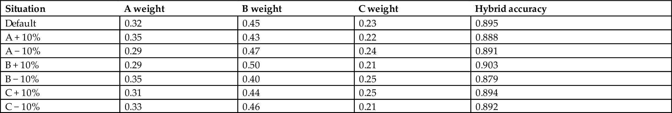
The sensitivity to a ± 10% change in A is − 0.7% and − 0.4%; to a ± 10% change in B, it is + 0.08% and − 1.6%; and to a ± 10% change in C, it is − 0.1% and − 0.3%. Please see text for details.
The results for these + 10 and − 10% changes in the weightings of the three Classifiers A, B, and C are shown in Table 5.1. The values are calculated as follows: The weight of the classifier that is to be changed is increased by 10% or decreased by 10%, and the remaining weights are then adjusted, so the sum of weights is still 1.0 (normalized). So, when the A weight moves from 0.32 to 0.35 (+ 10%), B weight decreases to 0.43, and C weight decreases to 0.22, so the sum of 0.35 + 0.43 + 0.22 = 1.0. For B weight, 0.45 is replaced by 0.45/(0.45 + 0.23) multiplied by 0.65, which comes to 0.43.
The sensitivity to a + 10% change in A is − 0.7%, and to a − 10% change in A, it is − 0.4%; to a + 10% change in B, it is + 0.08%, and to a − 10% change in B, it is − 1.6%; and to a + 10% change in C, it is − 0.1%, and to a − 10% change in C, it is − 0.3%. The mean sensitivity is the percentage change in accuracy divided by the percentage change in the weight, which is therefore − 0.07 and − 0.04 for A, + 0.08 and − 0.16 for B, and − 0.03 and − 0.01 for C. From this, we see that the magnitude of the mean sensitivity to B is more than twice that of A and is six times that of C. So, the overall accuracy is most sensitive to the weighting of Classifier B, and there only the positive direction results in a positive effect on the weighted voting combination accuracy. In this simple example, then, the system can be optimized by changing the relative weighting of Classifier B positively.
The next step is to test various positive shifts of the weighting of B and assess the hybrid accuracy. For some new sets of {A,B,C} weighting based on continuing in the directions of “positive effects on accuracy,” we chose these weighting triples ={0.32,0.45,0.23}, {0.31,0.46,0.23}, {0.31,0.47,0.22}, {0.30,0.48,0.22}, {0.30,0.49,0.21}, {0.29,0.50,0.21}, {0.28,0.51,0.21}, and {0.28,0.52,0.20}. For these eight combinations, we measured that the hybrid accuracy was, respectively, 0.895, 0.896, 0.898, 0.904, 0.906, 0.903, 0.0903, and 0.901. Thus, the peak is accuracy = 0.906 for the weights {0.30,0.49,0.21}. Since this is the only positive direction for sensitivity, we have almost certainly found a better set of weights than the original set of {0.32, 0.45, 0.23}. Note that this optimization simultaneously considered the absolute, relative, and directional sensitivities of the coefficients.
5.5 Sensitivity analysis of the hybrid algorithmics
Moving up a level, from the level of individual algorithms cooperating for a solution to adding more meta-algorithmic (e.g., ensemble, hybrid, and combinatorial approaches) systems to an existing hybrid system, our sensitivity is now focused on the overall change in system behavior when a new meta-algorithm is added to the system.
In Table 5.2, we are looking at the sensitivity of a hybrid system to each of its components. The components could be individual algorithms along the lines of the example covered in the previous Section 5.5; however, the approach is generalizable to any combination of meta-algorithms in addition to any combination of algorithms.
Table 5.2
| Meta-algorithmic number | Meta-algorithmic number | |||||
| 1 | 2 | 3 | … | N | ||
| 1 | — | NA | NA | NA | NA | |
| 2 | 1 + 2 | — | NA | NA | NA | |
| 3 | 1 + 3 | 2 + 3 | — | NA | NA | |
| … | … | … | … | — | NA | |
| N | 1 + N | 2 + N | 3 + N | … | — | |
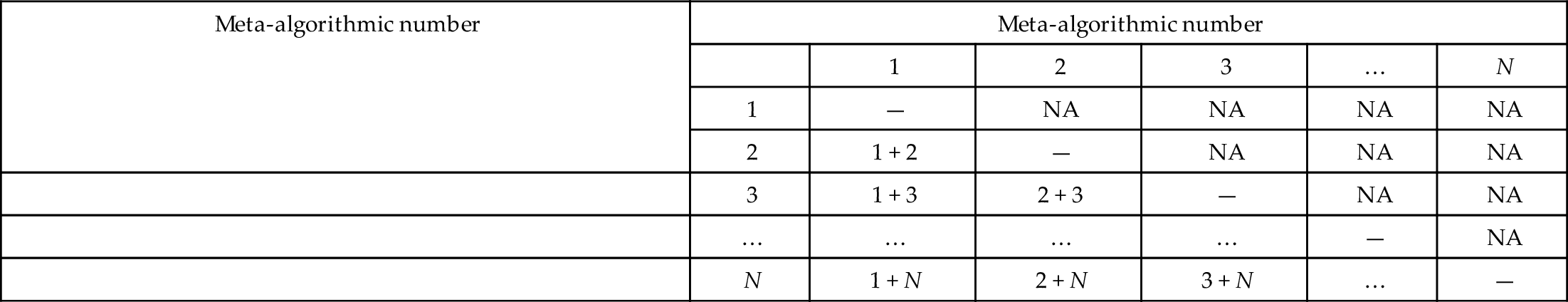
The comparisons made are indicated by “1 + 2,” “1 + 3,” etc., in the table. There are N(N − 1)/2 total comparisons to be made. Please see text for details.
We start with algorithms first. If, for example, we wished to explore adding another classifier, say Classifier E, to four classifiers already employed in a weighted voting pattern, then we might get the specific incarnation shown in Table 5.3. The table does not simply show what the weighted voting output is for Classifiers A + B + C + D and then A + B + C + D + E, which is important, but does not give a complete picture of the value of adding Classifier E. In the case of Table 5.3, it so happens that adding Classifier E improved the overall accuracy from 0.855 to 0.868, which is a 9.0% reduction in the error rate. But, more importantly, Table 5.3 can be used to assess the relative value of adding Classifier E to any of the other classifiers in the problem in several interesting ways. The first is to compute the peak sensitivity according to Eq. (5.12):
Table 5.3
| Meta-algorithmic number | Meta-algorithmic number | |||||
| A (0.822) | B (0.833) | C (0.755) | D (0.734) | E (0.714) | ||
| A (0.822) | — | NA | NA | NA | NA | |
| B (0.833) | 0.833 | — | NA | NA | NA | |
| C (0.755) | 0.838 | 0.844 | — | NA | NA | |
| D (0.734) | 0.844 | 0.829 | 0.812 | — | NA | |
| E (0.714) | 0.825 | 0.855 | 0.811 | 0.777 | — | |
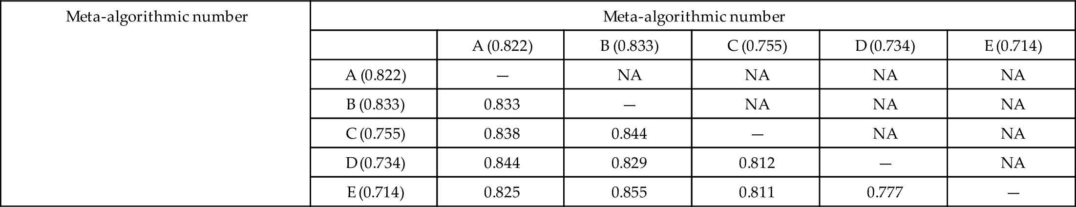
There are N(N − 1)/2 total comparisons to be made. Please see text for details. The values in parenthesis are the accuracies for each of the individual classifiers, while the table entries are the accuracies for the paired set of classifiers
In order to determine the peak sensitivity, we find the maximum difference between functions (accuracy being the “function” in this case) of two variables, subtracting the original function (accuracy) of one variable; for example, f(i,M)− f(M). For A, the peak sensitivity is for (D), since accuracy(A,D)− accuracy(A)=0.022. For B, the peak sensitivity is for (E), since accuracy(B,E)− accuracy(B)=0.022. For C, the peak sensitivity is for (B), since accuracy(B,C)− accuracy(C)=0.089. For D, the peak sensitivity is for (A), since accuracy(A,D)− accuracy(D)=0.110. Finally, for E, the peak sensitivity is for (B), since accuracy(B,E)− accuracy(E)=0.141. This is indeed the highest overall sensitivity, and importantly, the mean sensitivity of B and E is (0.022 + 0.141)/2 = 0.82. This is the highest overall sensitivity, implying that Classifiers B and E complement each other nicely. Thus, we have two methods for sensitivity analysis. The first is finding the classifier that best complements each classifier (this is peak sensitivity, or Eq. 5.12), and for {A,B,C,D,E}, this is {D,E,B,A,B}. We see that Classifier C is the only classifier that does not provide a peak sensitivity for any other classifier. Also, B and E provide the highest single (0.141) complement and the highest mean (0.82) complement pair. The mean complement by pair is thus the second sensitivity analysis metric from the table.
A third sensitivity analysis from the data in Table 5.3 is to find the mean and range of each classifier for complementing the other ones. For Classifier A, the mean is 0.76 (of 0.00, 0.083, 0.110, and 0.111), and the range is {0.00, 0.111}. The mean is thus the sum of the differences in the matrix for A with B, C, D, and E compared with the accuracy of B, C, D, or E alone and then divided by 4. For Classifier B, the mean is 0.84, and the range is {0.11, 0.141}. For Classifier C, the mean is 0.51, and the range is {0.11, 0.97}. For Classifier D, the mean is 0.35, and the range is {− 0.04, 0.63}—the negative value is because when D is added to B, it pulls the classification accuracy from B’s 0.833 to a combined 0.829. In general, this happens quite frequently, especially as our systems approach optimization. Finally, for Classifier E, the mean is 0.31, and the range is {0.03, 0.56}. Based on the means, the classifiers with the strongest “pull” (mean increase in accuracy when paired with another classifier) are, in order, B (pull = 0.79), A (pull = 0.76), C (pull = 0.51), D (pull = 0.35), and E (pull = 0.31). This happens to be the exact order of the individual classifiers for accuracy, which implies a generally correlated set of classifiers. However, we see that adding Classifier E, in spite of its relatively low accuracy, has a positive impact on each pairing with another classifier. This implies it should prove a robust addition to the overall classification.
Thus, we see how to use Table 5.1 for combining classifiers, each of which may by itself a meta-algorithm. For “pure” meta-algorithms, peak sensitivity is given by Eq. (5.12). Whether algorithms or meta-algorithms are being assessed, the number of comparisons to be made for the sensitivity analysis is N(N − 1)/2 where N = the number of meta-algorithmic patterns being considered for adding into the system.
5.6 Sensitivity analysis of the path to the current state
The final topic in sensitivity analysis to be covered here is related to path. This has a lot of applications, particularly in its use in Markov models and Bayesian networks. We start off considering its application to the Markov model originally presented in Section 1.7.3. In Table 5.4, we see all of the transition probabilities for the four-state system. In specific, we will be interested in the “no change” state-state transitions, that is, A➔A, B➔B, C➔C, and D➔D, with probabilities 0.33, 0.12, 0.26, and 0.22, respectively.
Table 5.4
| State n | |||||
| State n − 1 | A | B | C | D | |
| A | 0.33 | 0.25 | 0.22 | 0.20 | |
| B | 0.33 | 0.12 | 0.23 | 0.32 | |
| C | 0.28 | 0.24 | 0.26 | 0.22 | |
| D | 0.39 | 0.19 | 0.19 | 0.23 | |
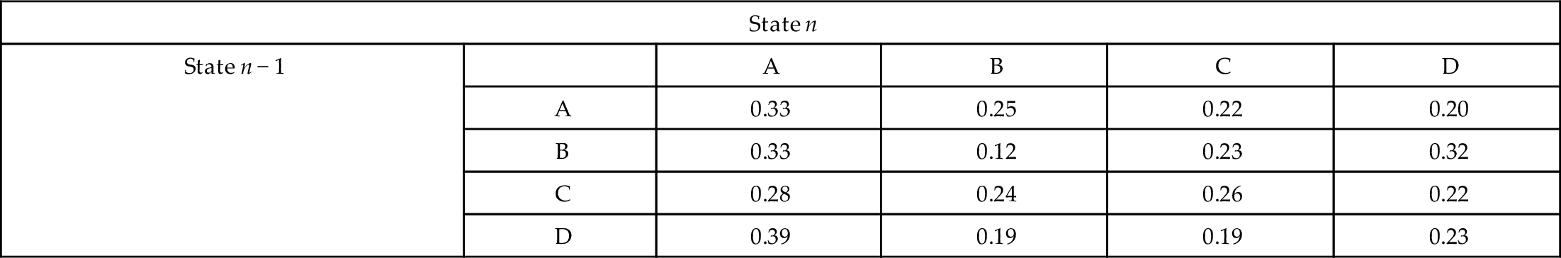
This is the starting point for the sensitivity analysis shown in Table 5.5 and described in the text.
In Table 5.4, note that each row sums to 1.0, as it must since the next state is always either A, B, C, or D. The columns do not have to sum to 1.0, and rarely do, but do give us a relative estimate of what percentage of time the system spends in each state. A closed-form solution of the Markov model is not available, so for the data of Table 5.4 (and later Table 5.5), the percentages are the means of three separate trials with 107 consecutive states.
Table 5.5
| Condition of the test | A pct (delta) | B pct (delta) | C pct (delta) | D pct (delta) |
|---|---|---|---|---|
| Original (see Table 5.4) | 0.3331 | 0.2067 | 0.2239 | 0.2363 |
| AA = 0.36, AB = 0.24, AC = 0.21, AD = 0.19 | 0.3433 (+ 0.0102) | 0.2039 (− 0.0028) | 0.2203 (− 0.0036) | 0.3433 (+ 0.0102) |
| AA = 0.30, AB = 0.26, AC = 0.23, AD = 0.21 | 0.3233 (− 0.0098) | 0.2094 (+ 0.0027) | 0.2272 (+ 0.0033) | 0.2401 (+ 0.0038) |
| BB = 0.15, BA = 0.32, BC = 0.22, BD = 0.31 | 0.3311 (− 0.0020) | 0.2124 (+ 0.0057) | 0.2218 (− 0.0021) | 0.2348 (− 0.0015) |
| BB = 0.09, BA = 0.34, BC = 0.24, BD = 0.33 | 0.3349 (+ 0.0018) | 0.2013 (− 0.0054) | 0.2261 (+ 0.0022) | 0.2377 (+ 0.0014) |
| CC = 0.29, CA = 0.27, CB = 0.23, CD = 0.21 | 0.3302 (− 0.0029) | 0.2048 (− 0.0019) | 0.2311 (+ 0.0072) | 0.2339 (− 0.0024) |
| CC = 0.23, CA = 0.29, CB = 0.25, CD = 0.23 | 0.3357 (+ 0.0026) | 0.2085 (+ 0.0018) | 0.2170 (− 0.0069) | 0.2387 (+ 0.0024) |
| DD = 0.26, DA = 0.38, DB = 0.18, DD = 0.180 | 0.3312 (− 0.0019) | 0.2044 (− 0.0023) | 0.2210 (− 0.0029) | 0.2433 (+ 0.0070) |
| DD = 0.20, DA = 0.40, DB = 0.20, DD = 0.20 | 0.3348 (+ 0.0017) | 0.2091 (+ 0.0024) | 0.2265 (+ 0.0026) | 0.2296 (− 0.0067) |
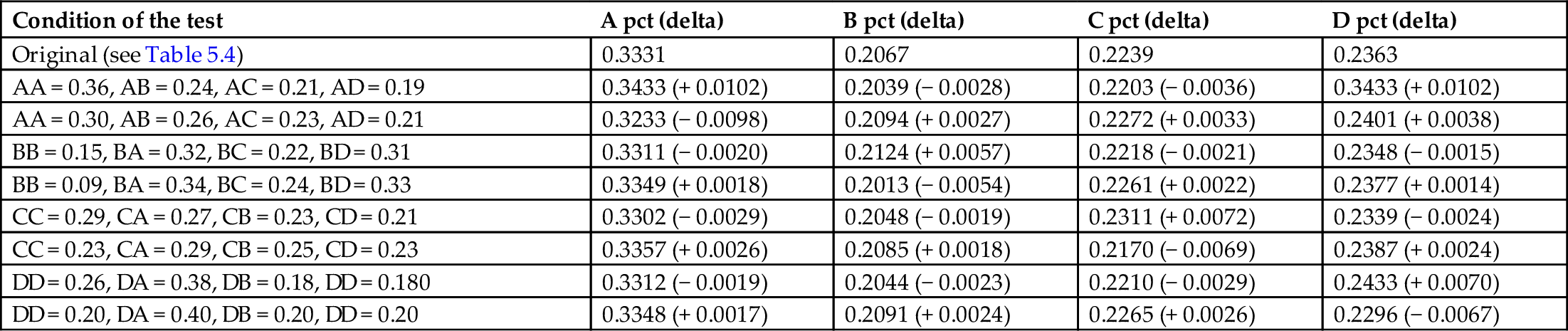
The tests performed were to add and subtract the margin of error (1.96 standard deviations, or 0.03) to the “steady-state” values of AA, BB, CC, and DD, respectively and distribute the delta evenly across the remaining three state-state transitions, as shown in the first column. The effects on the overall time spent in each state are shown in parentheses. Please see text for more details.
In Table 5.5, we carry out the sensitivity analysis using the “steady-state” situations of having state n − 1 and state n be the same. We could have used any other variation, for example, changing any of the 16 transition probabilities in Table 5.4 in both a positive and negative direction. For the purposes of illustration, though, we will simply change the four probabilities AA, BB, CC, and DD (steady-state staying at states A, B, C, and D, respectively) by + 3% and separately by − 3%. When this occurs, we must adjust the other probabilities downward, and so, for example, we decrease each of AB, AC, and AD probabilities by − 1% when AA is increased 3% and increase each of AB, AC, and AD probabilities by + 1% when AA is decreased 3%.
The results of each of these + 3% and − 3% variations are shown in Table 5.5. Sensitivity is measured based on the effect of adding or subtracting 3% of the times a state remains in state for the next iteration. The expected impact of the sensitivity is the variation added multiplied by the percentage of time spent in a given state. Since the variation is ± 3% and the percentage of time spent in the states A, B, C, and D (from the first data row in Table 5.5) is 0.3331, 0.2067, 0.2239, and 0.2363, respectively, then we expect the change on percent time spent at A, B, C, and D to be 0.0100, 0.0062, 0.0067, and 0.0071, respectively. As we see in Table 5.5, the mean effects on state A are 0.0100 (exactly as expected), the mean effects on state B are 0.0056 (lower than expected), the mean effects on state C are 0.0071 (higher than expected), and the mean effects on state D are 0.0069 (roughly as expected). Sensitivity is defined as the mean effect on the state (of the + and the − variability added divided by 2), divided by the percent of the time in the particular state, per Eq. (5.13):
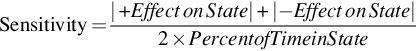
From Eq. (5.13), the sensitivity of AA =(0.0102 + 0.0098)/(2⁎0.3331)=0.0300, the sensitivity of BB =(0.0057 + 0.0054)/(2⁎0.2067)=0.0268, the sensitivity of CC =(0.0072 + 0.0069)/(2⁎0.2239)=0.0315, and the sensitivity of DD =(0.0070 + 0.0067)/(2⁎0.2363)=0.0290. Values above 0.03 (the ± variability added) are higher than predicted (this is true of CC), and values below 0.03 are lower than predicted (this is true of BB). We see from this set of results that state C is the one upon which the output is most sensitive. It makes sense for us, then, to focus on making sure that state C is made as predictable as possible (for cost, throughput, performance, accuracy, or whatever else is being measured or managed at each state) to best improve the predictive power of the overall system.
Markov chains are also readily amenable to path sensitivity analysis. Suppose we have a Markov chain A➔B➔C and we wish to calculate the probability of this path. The probability is p(A | BC)× p(B | C)× p(C). The overall sensitivity of the chain’s probability is therefore a function of the uncertainly of p(A | BC), p(B | C), and p(C). We use this to compare two close results, for example, p(ABC) and p(ACB). Suppose p(A | BC) is 20 ± 4%, p(B | C) is 40 ± 10%, and p(C) is 30 ± 6%. Then, suppose p(A | CB) is 19 ± 3%, p(C | B) is 38 ± 5%, and p(B) is 31 ± 3%. We see that p(ABC) = 0.0240 ± 0.0192 and p(ACB) = 0.0224 ± 0.0098. Clearly, we see that p(ABC) > p(ACB), but p(ABC) could be as low as 0.0048, and p(ACB) is never lower than 0.0126. If it is catastrophic from a process standpoint (quality control, risk assessment, etc.) to be below a certain value, for example, 0.0075 or 0.0100, then we may choose p(ACB) as the best path or sequence.
5.7 Summary
This chapter began with a review of sensitivity analysis approaches overviewed in this chapter and Chapters 6–14, elaborating further on the use of sensitivity analysis to assign individual models to portions of the domain for hybrid models. A deeper consideration of how many critical points to use for feature selection (initially introduced in Sections 1.10 and 1.11) was provided and later shown to be useful for destabilizing data groups with less entropy than other groups with which it will be analyzed. Destabilization was discussed for four situations: (a) when one set of ground truth has largely different entropy than the other sets, (b) when one set of ground truth is more or less discretized than the other sets, (c) when one set of ground truth is created by different means than the other sets, and (d) when the grouped behavior of the data is too similar by analytic evaluation.
Sensitivity analysis was then applied to a solution model. In linear system theory, the coefficients of the transfer function can be monitored for their variability over time directly, since the numerator and denominator both have linear equations. Sensitivity for a system of multiple equations is determined from the A matrix elements in the equation x(n + 1)= Ax(n)+ b.
Sensitivity analysis of individual algorithms in an ensemble, combinatorial, or other hybrid system was considered in Table 5.1. By varying the weights in a weighted voting system, we could compute absolute, relative, and directional effects. In our example, only one direction of sensitivity resulted in improved overall accuracy. This allowed us to focus on this direction for optimizing the overall system, in the end achieving an additional 1.1% in accuracy and reducing the error by 10.5% of its initial value.
A matrix approach to sensitivity analysis was used to determine if adding another algorithm or meta-algorithm is as effective as the combinations that have already been performed in a hybrid design. Three types of sensitivity—peak sensitivity of the combinations or maximum complement pairing, mean complement by pair, and mean and range of complementing—are computed for each of the multiple algorithms/meta-algorithms, and any anomalous behavior can be discerned.
Finally, sensitivity analysis of path was overviewed. This approach was shown to be particularly applicable to Markov models and Bayesian networks. We revisited the Markov model from Chapter 1 and showed how sensitivity analysis can point us to focus on the measurements upon which the final outputs are most sensitive.