You can use formulas to perform all kinds of calculations on your Excel data. You can build formulas using mathematical operators, values, and cell references. For example, you can add the contents of a column of monthly sales totals to determine the cumulative sales total. If you are new to writing formulas, this task explains all of the basics required to build your own formulas in Excel.
Formula Structure
Ordinarily, when you write a mathematical formula, you write the values and the operators, followed by an equal sign, such as 2+2=. In Excel, formula structure works a bit differently. All Excel formulas begin with an equal sign (=), such as =2+2. The equal sign immediately tells Excel to recognize any subsequent data as a formula rather than as a regular cell entry.

Referencing Cells
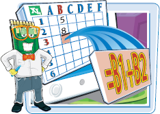
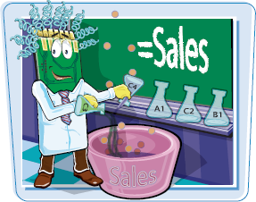
Although you can enter specific values in your Excel formulas, you can also easily reference data in specific cells. For example, you can add two cells together or multiply the contents of one cell by a value. Every cell in a worksheet has a unique address, also called a cell reference. By default, cells are identified by their specific column letter and then by their row number, and so cell D5 identifies the fifth cell down in column D. To help make your worksheets easier to use, you can also assign your own unique names to cells. For example, if a cell contains a figure totaling weekly sales, then you might name the cell Sales.
Cell Ranges
A group of related cells in a worksheet is called a range. Excel identifies a cell range by the anchor points in the upper-left and lower-right corners of the range. The range reference includes both anchor points separated by a colon. For example, the range name A1:B3 includes cells A1, A2, A3, B1, B2, and B3. You can also assign unique names to your ranges to make it easier to identify their contents. Range names must start with a letter or underscore, and can include uppercase and lowercase letters. Spaces are not allowed in range names.

Mathematical Operators
You can use mathematical operators in Excel to build formulas. Basic operators include the following:
Operator | Operation |
|---|---|
+ | Addition |
- | Subtraction |
* | Multiplication |
/ | Division |
% | Percentage |
^ | Exponentiation |
= | Equal to |
< | Less than |
≤ | Less than or equal to |
> | Greater than |
≥ | Greater than or equal to |
<> | Not equal to |
Operator Precedence
Excel performs a series of operations from left to right, but also gives some operatorsprecedence over others, as follows:
First | All operations enclosed in parentheses |
Second | Exponential equations |
Third | Multiplication and division |
Fourth | Addition and Subtraction |
When you are creating equations, the order of operations determines the results. For example, if you want to determine the average of values in A2, B2, and C2, and you enter the equation =A2+B2+C2/3, you will calculate the wrong answer. This is because Excel divides the value in cell C2 by 3 and then adds that result to A2+B2. Following operator precedence, division takes precedence over addition. The orrect ay to write the formula is =(A2+B2+C2)/3. By enclosing the values in parentheses, Excel adds the cell values first before dividing them by 3.
Reference Operators
You can use Excel's reference operators to control how a formula groups cells and ranges in order to perform calculations. For example, if your formula needs to include the cell range D2:D10 and cell E10, you can instruct Excel to evaluate all of the data contained in these cells using a reference operator. Your formula might look like this: =SUM(D2:D10,E10).
Operator | Example | Operation |
|---|---|---|
: | =SUM(D3:E12) | Range operator. Evaluates the reference as a single reference, including all of the cells in the range from both corners of the reference. |
, | =SUM(D3:E12,F3) | Union operator. Evaluates the two references as a single reference. |
[space] | =SUM(D3:D20 D10:E15) | Intersect operator. Evaluates the cells common to both references. |
[space] | =SUM(Totals Sales) | Intersect operator. Evaluates the intersecting cell or cells of the column labeled Totals and the row labeled Sales. |
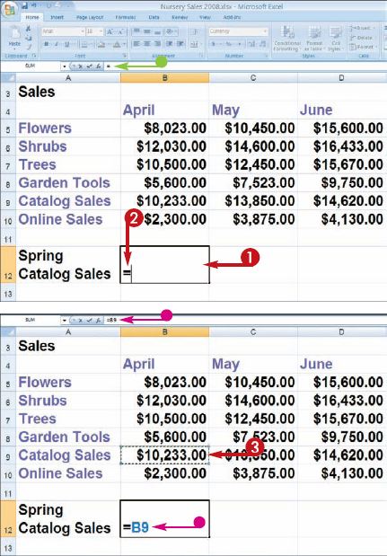
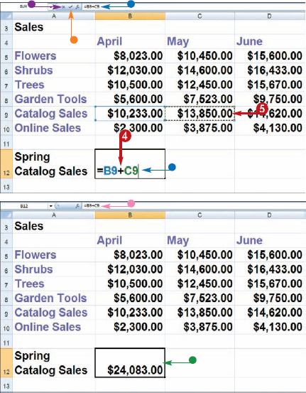
You can write a formula to perform a calculation on data in your worksheet cells. All formulas begin with an equal sign (=) in Excel. You can reference values in cells by entering the cell name, also called a cell reference. For example, if you want to add the contents of cells C3 and C4 together, your formula looks like this: =C3+C4.

You can create a formula in the Formula bar at the top of the worksheet. Formula results appear in the cell to which you assign a formula.
Create Formulas
Note
See the previous task, "Understanding Formulas," to learn more about mathematical operators
To view the formula in the Formula bar, you can simply click in the cell.
Note
If you change any of the values in the cells referenced in your formula, the formula results automatically update to reflect the changes.
Note
How do I edit a formula?
To edit a formula, simply click in the cell containing the formula and make any corrections in the Formula bar. You can also double-click in the cell to make edits directly to the formula within the cell. You can use the keyboard arrow keys to move the cursor to the place you want to edit in the data, or simply click the cursor in place. You can press

What happens if I see an error message in my formula?
If you see an error message, such as #DIV/0!, double-check your formula references to ensure that you referenced the correct cells. Also make sure that you did not attempt to divide by zero, which always produces an error. To learn more about fixing formula errors, see the "Audit a Worksheet for Errors" task, later in this chapter.SSTTOOPP


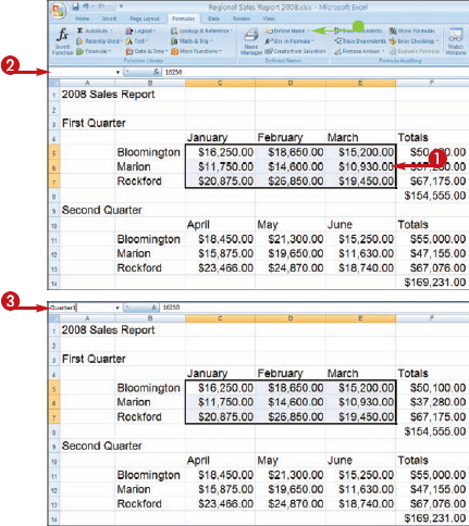
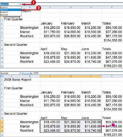
You can assign distinctive names to the cells and ranges of cells that you work with in a worksheet, making it easier to identify the cell'scontents. A range is simply a rectangular group of related cells; a range can also consist of a single cell. Naming ranges can also help you when deciphering formulas. A range name, such as Sales_Totals, is much easier to recognize than a generic reference, such as B24:C24.
Define a Range Name
ASSIGN A RANGE NAME
Excel assigns the name to the cells.
GO TO A RANGE
Note
Are there any rules for naming ranges?
Yes. Range names must start with a letter or an underscore (_). After that, you can use any character, uppercase or lowercase, or any punctuation or keyboard symbols, with the exception of a hyphen or space. Because neither hyphens nor spaces are allowed in range names, you can substitute them with a period or underscore.

How do I edit a range name?
You can use the Name Manager feature to make changes to your range names. To display the Name Manager, click the Name Manager button on the Formulas tab. You can edit existing range names, change the cells referenced by a range, or remove ranges to which you no longer need names assigned in the worksheet.

You can reference an entire group of cells in a formula by referencing its range name. This can speed up the time it takes to build a formula in a worksheet, and range names are much easier to remember than the default range names that Excel assigns.
Reference Ranges in Formulas
Note
See the "Create Formulas" task, earlier in this chapter, to learn more.
Excel automatically inserts the range name.
You can also select the range directly in the worksheet.
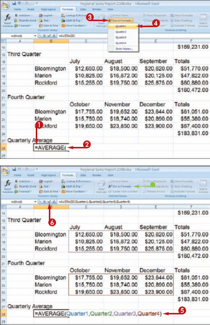
The formula results appear in the cell.
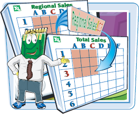
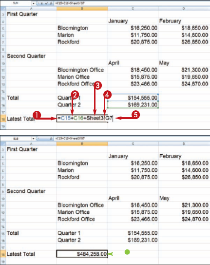
You can reference cells in other worksheets in your Excelormulas. When referencing data from other worksheets, you must specify the worksheet name, followed by an exclamation mark and then by the cell address, such as S heet2!D12. If the worksheet has a specific name, such as Sales, you must use the name along with an exclamation mark, followed by the cell or range reference (Sales!D12). If the worksheet name includes spaces, enclose the reference in single quote marks, such as 'Sales Totals!D12'.
See Chapter 10 to learn more about naming Excel worksheets.
Reference Cells from Other Worksheets
Note
See the "Create Formulas" task, earlier in this chapter, to learn more.
You can continue creating the formula as needed.
By default, Excel treats the cells that you include in formulas as relative locations rather than set locations in the worksheet. This is called relative cell referencing. For example, when you copy a formula to a new location, the formula automatically adjusts using relative cell addresses. If you want to address a particular cell location no matter where the formula appears, you can assign an absolute cell reference. Absolute references are preceded with a dollar sign in the formula, such as =$D$2+E2.

Apply Absolute and Relative Cell References
ASSIGN ABSOLUTE REFERENCES
Note
You can also type dollar signs to make a reference absolute.
Note
You can continue pressing
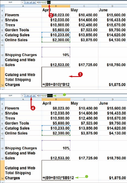
Excel assigns the changes to the formula.
ASSIGN RELATIVE REFERENCES
Note
You can press
Note
You can also type dollar signs to make a reference absolute.
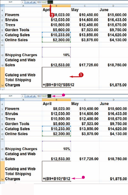
Note
When would I use absolute cell references?
You can use absolute referencing to always refer to the same cell in a worksheet. For example, perhaps your worksheet contains several columns of pricing information that refer to one discount rate disclosed in cell G10. When you create a formula based on the discount rate, you want to make sure that the formula always refers to cell G10, even if the formula is moved or copied to another cell. By making cell G10 absolute instead of relative, you can always count on an accurate value for the success of your formula.

When would I use mixed cell references?
You can use mixed referencing to reference the same row or column, but different relative cells within, such as $C6, which keeps the column from changing while the row remains relative. If the mixed eference is C$6, the column is relative but the row is absolute. You can press

If you are looking for a speedier way to enter formulas, you can use a wide variety of built-in formulas, called functions. Functions are ready-made formulas that perform a series of operations on a specified range of values. Excel offers over 300 functions that you can use to perform mathematical calculations on your worksheet data.
Function Elements
Because functions are formulas, all functions must start with an equal sign (=). Functions are also distinct in that each one has a name. For example, the function that sums data is called the SUM function, while the function for averaging values is called the AVERAGE function. You can type functions directly into your worksheet cells or into the Formula bar. You can also use the Insert Function dialog box to help construct functions. This dialog box offers help in selecting and applying functions to your data.

Constructing Arguments
Functions typically use arguments to indicate the cell addresses that you want the functions to calculate. Arguments are enclosed in parentheses. When applying a function to individual cells in the worksheet, you can use a comma to separate the cell addresses, such as =SUM(A5,B5,C5). When applying a function to a range of cells, you can use a colon to designate the first and last cells in the range, such as =SUM(B5:E12). If your range has a name, you can insert the name, such as =SUM(Sales).

Types of Functions
Excel groups functions into ten categories, and each category can include a variety of functions:
Category | Description |
|---|---|
Database & List Management | Includes functions for counting, adding, and filtering database items. |
Date & Time | Includes functions for calculating dates, times, and minutes. |
Engineering | Offers many kinds of functions for engineering calculations. |
Financial | Includes functions for calculating loans, principal, interest, yield, and depreciation. |
Information | Includes functions for testing your data. |
Logical | Includes functions for logical conjectures, such as if-then statements |
Lookup & Reference | Includes functions that enable you to locate references or specific values in your worksheets. |
Mathematical & Trigonometric | Includes a wide variety of functions for calculations of all types. |
Statistical | Includes functions for calculating averages, probabilities, rankings, trends, and more. |
Text | Includes text-based functions to search and replace data and other text tasks. |
Common Functions
The table below lists some of the more popular Excel functions that you might use with your own spreadsheet work.
Function | Category | Description | Syntax |
|---|---|---|---|
SUM | Math & Trig | Math & Trig | =SUM(number1,number2,...) |
INT | Math & Trig | Rounds down to the nearest integer | =INT(number) |
ROUND | Math & Trig | Rounds a number specified by the number of digits | =ROUND(number,number_digits) |
ROUNDDOWN | Math & Trig | Rounds a number down | =ROUNDDOWN(number,number_digits) |
COUNT | Statistical | Returns a count of text or numbers in a range | =COUNT(value1,value2,...) |
AVERAGE | Statistical | Averages a series of arguments | =AVERAGE(number1,number2,...) |
MIN | Statistical | Returns the smallest value in a series | =MIN(number1,number2,...) |
MAX | Statistical | Returns the largest value in a series | =MAX(number1,number2,...) |
MEDIAN | Statistical | Returns the middle value in a series | =MEDIAN(number1,number2,...) |
PMT | Financial | Finds the periodic payment for a fixed loan | =PMT(interest_rate,number_of_periods,present_value,future_value,type) |
RATE | Financial | Returns an interest rate | =RATE(number_of_periods,payment, present_value,future_value,type,guess) |
TODAY | Date & Time | Returns the current date | =TODAY() |
IF | Logical | Returns one of two results that you specify based on whether the vis TRUE or FALSE AND | =IF(logical_text,value_if_true, value_if_false) |
AND | Logical | Returns TRUE if all of the arguments are true, FALSE if any are false | =AND(logical1,logical2,...) |
OR | Logical | Returns TRUE if any argument is true or FALSE if all arguments are false | =OR(logical1,logical2,...) |
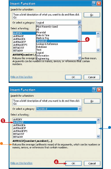
You can use functions to speed up your Excel calculations. You can use the Insert Function dialog box to look for a particular function from among Excel's ten function categories.

Apply a Function
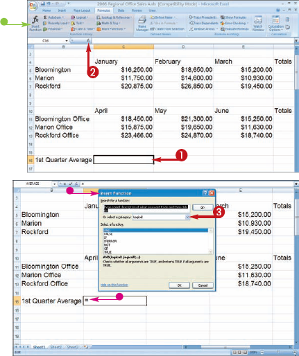
Excel's built-in functions are grouped into ten categories.
Note
See the previous task, "Understanding Functions," to learn 4 more about function categories.
Note
What kind of results can I expect with Excel functions?
Most of the time, the functions that you create will produce number results. However, because functions use different types of arguments, some functions produce different types of results.
Result | Description |
|---|---|
Number | Number results can include any integer or decimal number. |
Time & | Provides time and date results. |
Logical values | Logical arguments produce results such as TRUE, FALSE; YES, NO; 1, 0. |
Text | Any text results always appear surrounded by quotation marks. |
Arrays | An array is a column or table of cells that are treated as a singlem value, and array formulas operate on multiple cells. |
Cell references | Some function results display references to other cells rather than actual values. |
Error values | If a function uses error values as arguments, the results appear as error values as well. Error values are not the same as error messages |
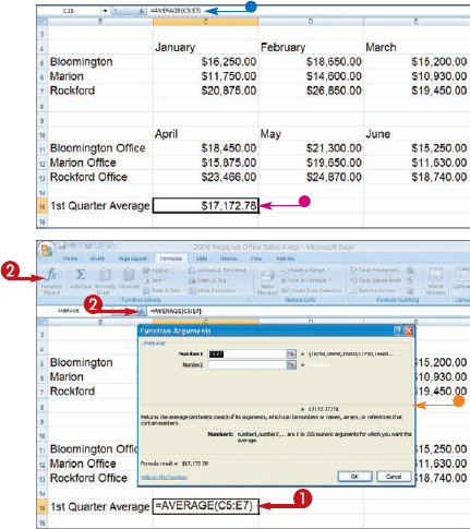
After selecting a function, you can then apply the function to a cell or range of cells in your worksheet. You can use the Function Arguments dialog box to help you construct all of the necessary components of a function. The dialog box can help you to determine what values you need to enter to build the formula.

The Function Arguments dialog box appears.
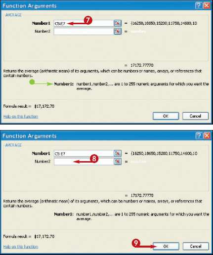
If you select a cell or range of cells directly in the worksheet, Excel automatically adds the references to the argument.
You can also type a range or cell address into the argument text box.
EDIT A FUNCTION
Note
How can I find help with a particular function?
If you click the Help on this function link in either the Insert Function or Function Arguments dialog box, you can access Excel's Help files to find out more about the function. The function help includes an example of the function being used, and tips about how to use the function.

The Function Arguments dialog box covers the cells that I need to select. How do I move the dialog box out of the way?
You can click the Collapse button (

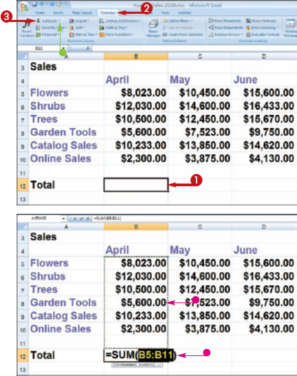
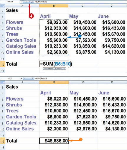
One of the most popular functions available in Excel is the AutoSum function. AutoSum automatically totals the contents of cells. For example, you can quickly total a column of sales figures. AutoSum works by guessing which surrounding cells you want to total, although you can also specify exactly which cells to sum.

Total Cells with AutoSum
You can also click the AutoSum button on the Home tab.
Note
Can I total cells without applying a function?
Yes. Excel's status bar quickly sums cells or displays results from several other popular functions without having to insert a formula or function into a cell. When you select a group of cells that you want to total, Excel immediately adds all of the cell contents and displays a total in the status bar at the bottom of the program window. To sum noncontiguous cells, press and hold

Can I apply AutoSum to both rows and columns at the same time?
Yes. Simply select both the row and column of data that you want to sum, along with a blank row and column to hold the results. When you apply the AutoSum function, Excel sums the row and column and displays the results in the blank row and column.


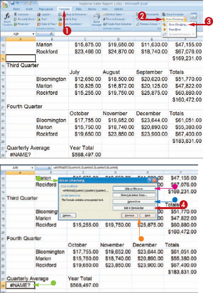
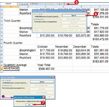
When dealing with larger worksheets in Excel, it is not lways easy to locate the source of a formula error when scrolling through the many cells. To help you with errors that arise, you can use Excel's ormula Auditing tools to examine and correct formula errors. The Error Checking feature looks through your worksheet for errors and helps you find Solutions.
Audit a Worksheet for Errors
APPLY ERROR CHECKING
Note
What kinds of error messages does Excel display for formula errors
The following table explains some of the different types of error values that can appear in cells when an error occurs:
Error Message | Error Message | Solution |
|---|---|---|
###### | The cell is not wide enough to contain the value | Increase the column width |
#DIV/0! | Dividing by zero | Edit the cell reference or value of the denominator |
#N/A | Value is not available | Ensure that the formula references the correct value |
#NAME? | Does not recognize text in a formula | Ensure that the name referenced is correct |
#NULL! | Specifies two areas that do not intersect | Check for an incorrect range operator or correct the intersection problem |
#NUM! | Invalid numeric value | Check the function for an unacceptable argument |
#REF! | Invalid cell reference | Correct cell references |
#VALUE! | Wrong type of argument or operand | Double-check arguments and operands |
Auditing tools can trace the path of your formula components and check each cell reference that contributes to the formula. When tracing the relationships between cells, you can display tracer lines to find precedents, cells referred to in a formula, or dependents, cells that contain the formula results.

PRECEDENTS
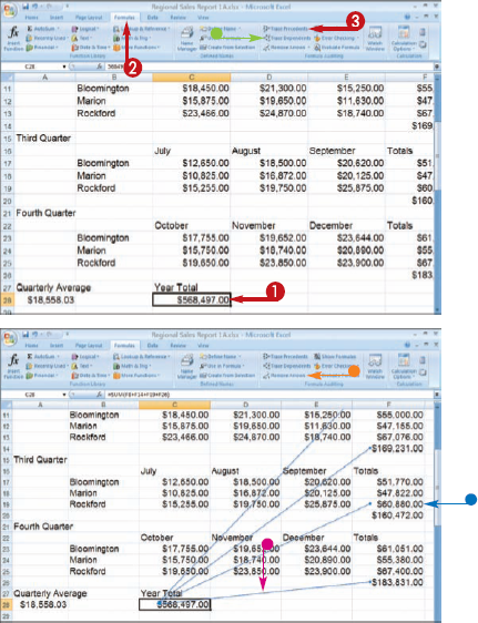
You can make changes to the cell contents or to the formula to make any corrections.
TRACE ERRORS
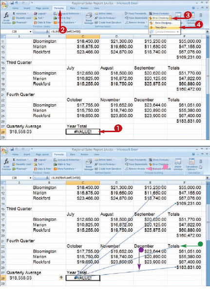
You can make changes to the cell contents or changes to the formula to correct the error.
Note
How do I use the Smart Tag to fix formula errors
Excel displays a Smart Tag icon (

What does the Evaluate Formula button do?
You can click the Evaluate Formula button (

