![]()
Microsof t Azure Machine Learning
Machine Learning emphasizes the computational work of software to process sample and/or historic data with the goal of uncovering interesting patterns, identifying objectives, and predicting outcome. For example, machine learning might uncover that for the past 14 years of worker’s compensation claims data, ear injuries in construction have an 88% chance of staying open for 180 days. Or when provided with juvenile offender historic data and recent juvenile crime data, machine learning might predict a 79% chance that a given juvenile’s next offense will result in an assault.
What Is Microsoft Azure Machine Learning?
Microsoft Azure Machine Learning (ML) is an advanced analytics cloud platform that makes it easy to design, test, deploy, and share powerful and predictive analytics. Microsoft Azure Machine Learning lets you build analytical experiments and predictive models. A rich set of algorithms can be used to process data based on business needs. Azure Machine Learning also provides tight integration with the public domain languages R, Python, and SQLite. And because Azure Machine Learning lives in the cloud, the platform has inherent scalability, availability, and security.
R is an industry favorite of data scientists and statisticians. R includes a rich scripting language to manipulate, statistically analyze, and visualize data. Python is an open source programming language that makes it easy to develop powerful and comprehensive programs. SQLite, in addition to being a development platform, provides a SQL language with which most relational database administrators are already very familiar.
Once the Azure Machine Learning experiment has been tested and evaluated, you can deploy a fully managed web service with a few clicks and that can connect to data of all shapes and sizes. The Azure Machine Learning web services may be published to the Azure Marketplace, offering businesses the opportunity to provide predictive services for a fee.
Quick Hands-On Introduction
Before further education on the Azure Machine Learning capability it’s important to get familiar with some basic terms and workflow using the platform.
Follow these steps to sign-up for your Azure ML subscription. If you don’t have the time to do this now, the screen illustrations, descriptions, and walkthrough will still be educational:
- Browse to http://azure.com/ml as seen in Figure 14-1, and either click on Get started now
 and sign-up for an Azure Machine Learning subscription or click on Pricing and get a free one-month trial.
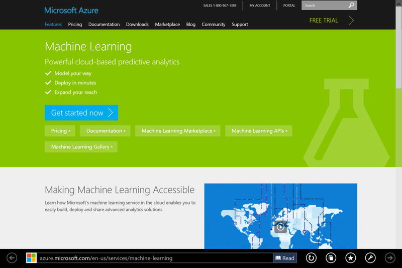
Figure 14-1. Azure Machine Learning Website
- From the Azure Portal, you will find the Azure Machine Learning icon along the left side (you may need to scroll down). Click on the icon shown in Figure 14-2.
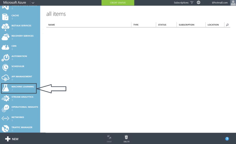
Figure 14-2. Azure Machine Learning in the Azure Portal
- Once you have clicked on the Machine Learning Icon, click on +NEW in the lower-left corner and follow the steps, as shown in Figure 14-3, to set up and then access your Azure Machine Learning workspace. (The Hotmail address in masked in this figure.)
Figure 14-3. Creating an Azure Machine Learning Workspace
Once complete, you should see a screen similar to Figure 14-4.
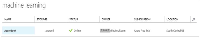
Figure 14-4. Azure Machine Learning Subscription
- From here, highlight your Azure workspace and at the bottom of the screen, click Open in Studio. Figure 14-5 depicts Azure Machine Learning Studio (ML Studio).
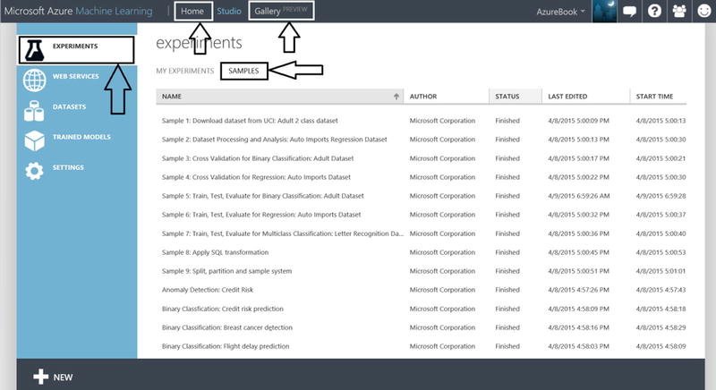
Figure 14-5. Azure Machine Learning Samples
 Note ML Studio is where you will spend the vast majority of your time. This is where your Azure machine learning experiment authoring, analysis, and deployment takes place. An Azure Machine Learning experiment is an authoring “container”, which encapsulates the data that you want to analyze, data cleansing you choose to perform, data feature selection, processing of algorithms against your data, validation of your analytics, prediction scoring and much more. You can copy, run, share experiments to other workspaces, and publish your experiment as a web service. Near the top of ML Studio you will find Gallery. This is where Microsoft and the Azure Machine Learning community (including you!) have shared experiments for others to investigate and incorporate. The experiments found in the gallery may include detailed write-ups, best practices and instructions for incorporating into your personal ML Studio workspace! Poke around in here and take a look at the various assets. Also near the top of ML Studio is where Home is. Go here to find a number of excellent learning resources.
 - You’ll notice in Figure 14-5 that there are a number of sample experiments that Microsoft has provided. Scroll around, select an experiment or two and get familiar with the way the various experiments have been authored on the design canvas.
- Now navigate to the experiment, “Sample 5: Train, Test, Evaluate for Binary Classification: Adult Dataset,” as shown in Figure 14-6. This experiment will process adult census data and predict whether an individual, based on demographic attributes, will have an income greater than $50,000, or less than or equal to $50,000.
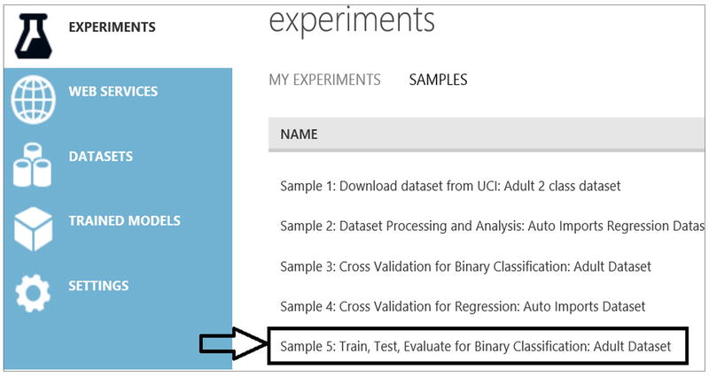
Figure 14-6. Azure Machine Learning Sample Experiments
- Click to open the Sample 5 experiment. Then click Save As at the bottom of the screen, and name your experiment AdultCensusSalaryPrediction. You should see something that looks similar to Figure 14-7.
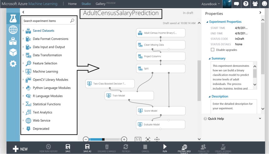
Figure 14-7. Machine Learning Census Experiment
- Click RUN at the bottom of the experiment to have Azure Machine Learning process the census data and crunch the numbers as directed by the data process flow.
Note If you want to play around with this experiment before continuing, then work with your own copy by saving it under a different name. Be sure to open and return to the AdultCensusSalaryPrediction experiment when you are ready to proceed.
Now that you have the AdultCensusSalaryPrediction experiment created from the sample, you can’t help but see the data flow and processing that is on the design canvas. What you are seeing on the canvas is called modules. These modules were dragged and dropped onto the canvas from the module list annotated in Figure 14-7 on the left side of the screen.
You can click on each major category of module and get a sense of the vast number of modules at your disposal. Once a module is dropped onto the canvas, you can connect their input and output ports to one another telling Azure Machine Learning how to process and direct the data as it winds through the data flow. Furthermore, you can have multiple independent data flow processing paths that will be run in parallel. You can cleanse data, split data, sample data, train algorithms on data, and score data with the probability of some desired outcome. You can also bring your favorite R scripts, Python, and SQLite into the mix.
- Investigate a module further. Click on any module on the canvas, and notice that its properties appear on the right side of the canvas.
- After an experiment is successfully run, the modules will have a green check mark status indicator at their right, as illustrated in Figure 14-8. If you do not see the green check marks in the modules, then click on RUN at the bottom of the screen.

Figure 14-8. Azure Machine Learning Module
- To see the dataset “Adult Census Income Binary…” that is being analyzed, click on its output port as illustrated in Figure 14-9.
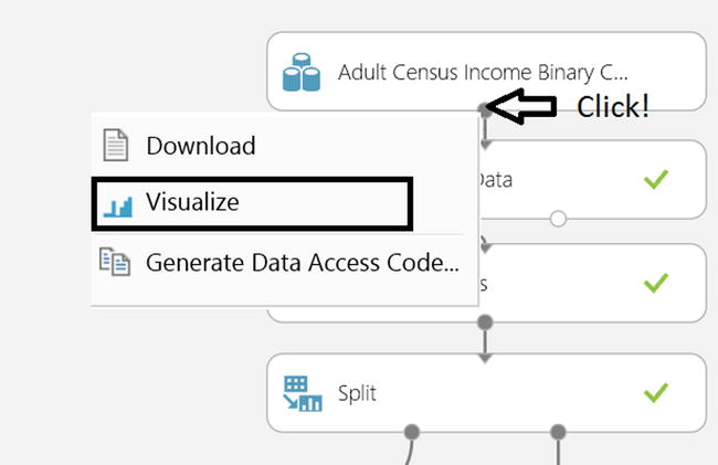
Figure 14-9. Machine Learning Data Cleansing Visualizations
- To look closely at the data, click Visualize and you will see the rows, columns and some basic charting for the census data being processed, as illustrated in Figure 14-10.
The census data looks similar to what is shown in Figure 14-10.
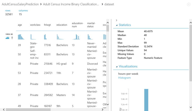
Figure 14-10. Census Data Visualizations
The census data incorporated in our experiment arrived there as a result of uploading a .csv file.
- To create a dataset by uploading a .csv file, click +NEW from the Home page in ML Studio. Now click on the three-cylinder DATASET icon illustrated in Figure 14-11. From here you can see where you would upload from a local file. There is no need to proceed any further with this step as the dataset has already been created.

Figure 14-11. Importing Datasets from CSV Files
![]() Note You can also bring data into an experiment using the Reader module. The Reader module can read data from Hadoop, SQL Azure Database, OData feeds, and so on.
Note You can also bring data into an experiment using the Reader module. The Reader module can read data from Hadoop, SQL Azure Database, OData feeds, and so on.
The Reader and Writer modules, as seen in Figure 14-12, will be very valuable as you author and design more sophisticated Azure Machine learning experiments.
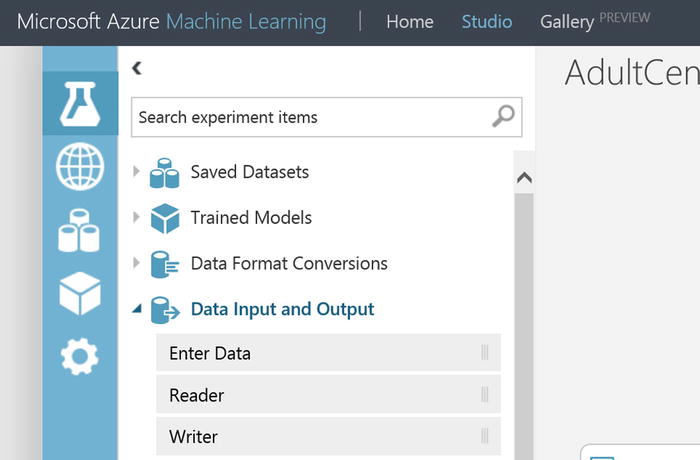
Figure 14-12. Reader and Writer modules within ML Studio
![]() Note A dataset that is saved by clicking a module’s output port and then selecting Save as Dataset can be accessed from any experiment, simply drop it onto the canvas as shown in Figure 14-13.
Note A dataset that is saved by clicking a module’s output port and then selecting Save as Dataset can be accessed from any experiment, simply drop it onto the canvas as shown in Figure 14-13.
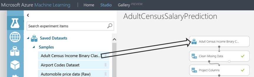
Figure 14-13. Adding Datasets to an Experiment
Now we will leave our quick hands-on peek into Azure Machine Learning and ML Studio. The experiment AdultCensusSalaryPrediction will be referenced as needed to support the educational process but it is not necessary for you to actively work in the experiment in ML Studio unless you would like to explore as we go along.
What Is a Good Machine Learning Problem?
The success of a machine learning solution is largely dependent on topical, consistent, and feature rich data. For machine learning to provide insight or predict outcome, it is very important to have quality representative data that captures past state for the predictions desired. Assume there is historical data for the income and demographics of people living between 1900 and 1920. The characteristics and demographics of a person making $50,000 dollars in the early 20th century would be of little value when faced with the exercise of predicting income for an individual living in 2015. Most predictive qualities around income for that data would be rather useless in predicting income today.
To predict the likelihood of an individual making more than $50,000 dollars, it will be necessary to have historical data that has a column representing the individual’s annual income. In the census dataset the column income classifies the individuals as making less than or equal to $50,000 (“<=50”) or greater than $50,000 (“>50”). The column income in machine learning vernacular is called a label column. A label may have multiple classes. The label income has two classes (“<=50”, “>50”) and those two classes are what the experiment AdultCensusSalaryPrediction will try to predict. The census data also has columns that are features supporting the label income.
A feature is a machine learning term that represents the columns of data that each provide some unique or independent characteristic supporting the label(s). For example, if there was a column Occupation with the value “clerk” and another column JobId with the value “c” and they both represented the same thing, then it would suffice to choose either Occupation or JobId as a feature in the experiment, but not both. In the census dataset examples of featuresAzure ML:education features are: Gender, Age, Education, and Marital Status. When a feature is categorical it contains some limited set of domain values, for example, the categorical feature Education has values such as Bachelors, HS-grad, 11th, 9th and so on.
The experiment AdultCensusSalaryPrediction is supported by a census dataset that includes one label with two classes and multiple features with respective domain values. However, it’s important to understand that machine learning problems and their associated Azure ML experiments can be extremely diverse. There could be experiments that operate on data that is highly numeric, or data that has multiple labels with numerous class values, perhaps data that is image data and so on. Figure 14-14 offers a glimpse into the csv file that makes up the census dataset. It has been annotated with machine-learning terms.
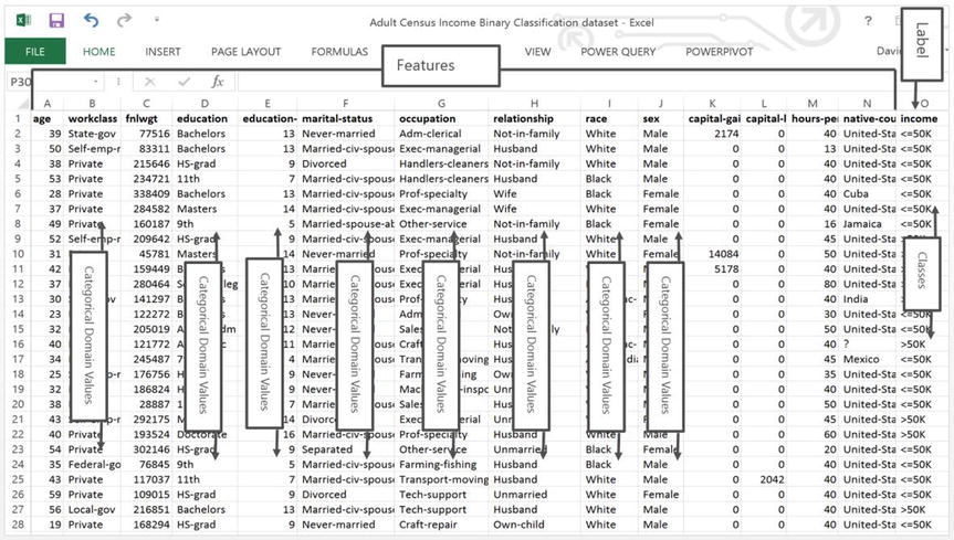
Figure 14-14. Census Data Cleansing in ML Studio
Ideally the dataset that ultimately flows into the algorithm(s), as directed by the Azure Machine Learning experiment, is cleansed of errors, missing values and less important features. Given such a dataset it is possible to train a model to predict and identify disease risk, a product marketing opportunity, transaction fraud, or predict adult income.
Data Cleansing and Preparation
In the experiment AdultCensusSalaryPrediction, illustrated in Figure 14-15, some data cleansing takes place through the Clean Missing Data module that resides on the canvas. The Clean Missing Data input port is connected to the output port of the raw census dataset. The Clean Missing Data module properties can be configured to indicate what happens when missing values are encountered. The module can remove an entire row from the data flow if a given column has a missing value, replace a numeric column with the mean of the values, replace a missing value with a custom value, or even calculate a value. The author can configure the properties to indicate what minimum missing value ratio must be met before any action is taken, same behavior for maximum missing value ratio.
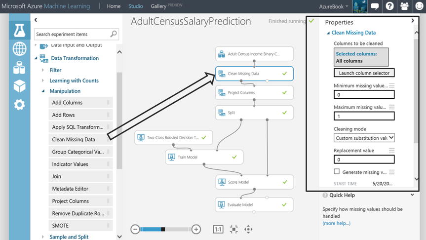
Figure 14-15. Census Data Cleansing in ML Studio
It is not uncommon that the majority of heavy lifting for a sound machine-learning project starts with data selection, feature engineering, data preparation and cleansing. This work can be done at the source, outside of Azure Machine Learning, or to some extent, inside the experiment using the various modules designed for data transformation. Data cleansing can also be carried out using the very powerful data manipulation aspects of the scripting modules for R, SQLite and Python.
There are a number of modules in ML Studio designed to cleanse and prepare data. For example, there is a commonly used module that allows the author to selectively pass along a subset of the columns to the data flow that might train an algorithm. The module to perform this operation is Project Columns and it is found on the AdultCensusSalaryPrediction experiment canvas. Notice how it has been hooked up to the data flow through its input and output ports respectively. The module’s Launch column selector found in the property pane on the right side of the canvas, as shown in Figure 14-16, is used to identify which columns are excluded or included as the data flows through the experiment.

Figure 14-16. Projecting Columns in ML Studio
In this experiment, and for the subsequent data flow, the Project Columns module excludes the columns: workclass, occupation, and native-country, as seen in Figure 14-17.
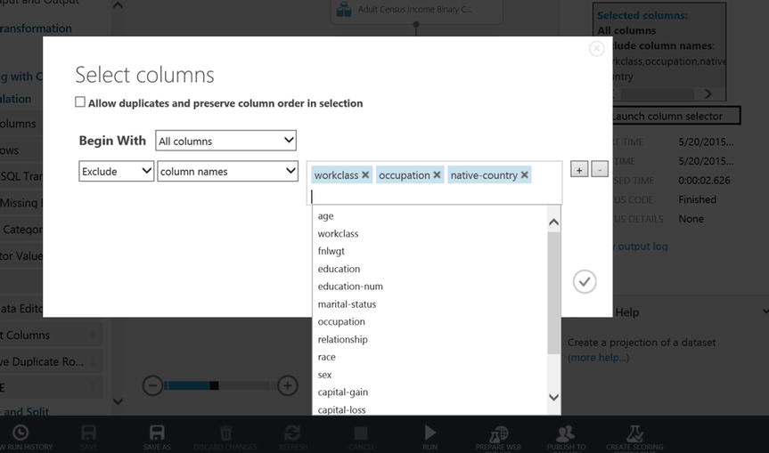
Figure 14-17. Excluding Columns in ML Studio
Choose an Algorithm and Train the Model
As a mental exercise and examining the census dataset, the goal is to predict an individual’s likelihood of making more than $50,000 dollars. Assume nothing is known about the algorithms. Given the census dataset and the classes “<=50” and “>50” along with the desire to predict “>50”, what would an approach be to look for aspects of the data that lean strongly to an individual making more than $50,000? One approach might be to use a tool like Excel and begin to chart, graph, grid, pivot, and group counts of features and their domain values until the most compelling features and values unveil themselves. Features and values that best influence the class “>50”. With patterns and correlations uncovered in Excel and given an individual and all their features, it would be possible to now see how that individual’s features and respective values fit into the hand-spun Excel analytics, which hopefully suggest a likelihood that the individual could be classified as “>50”. It’s important to point out that this Excel process could have been fraught with trial and error, human instinct, and false assumption. It is not to say that the conclusion of the Excel effort isn’t valid, but it is possible that hidden and interesting correlations went undiscovered or obvious correlations (or dependence and causality) weren’t accounted for. Machine learning will not only apply systematic and algorithmic mathematical rigor to this problem, it will do it in such a way that a person with Excel simply couldn’t keep up with the computational processing as the data is sorted, branched, grouped, calculated and iterated over and over again. This is what Azure Machine Learning is doing. Of course the proper algorithms need to be chosen and configured as appropriate, but there is nothing like having a number crunching machine as your partner when analyzing data!
With the power of Azure Machine Learning and the right algorithms to do the heavy lifting, not only can millions of rows of data be crunched, but the effort in classifying and predicting each individual as “<=50” or “>50” will be carried out with the complexity and mathematical rigor required to arrive at an answer. The experiment author chooses the right algorithm and Azure Machine Learning does the rest of the work.
Choosing algorithms can be tricky but to understand some basic algorithm types, consider these three major areas:
- Classification: Classify each training instance (row) by assigning it to some set of fixed values. For example, for each individual their income is classified as “<=50” or “>50”. For an insurance claim instance, it will be either TRUE or FALSE that the claim is open 180 Days. For street location and hour of day, the 911 event will be one of Disturbance, Violent, Liquor, Accident, or Other.
- Clustering: Partitions instances into similar groups. For example, group decedents based on cause of death, location, age, ethnicity, autopsy performed, and so forth. Within these groups, look for interesting patterns and correlations.
- Regression: Predict a real value for each instance. For example, predicting the speed for vehicle traffic, or predicting the cost of highway project types.
As the experiment AdultCensusSalaryPrediction is further inspected, notice that the data is split in Figure 14-18 so that the selected algorithm only uses a portion of the data. The remaining data will be used to evaluate the precision and accuracy of the model at a later point.
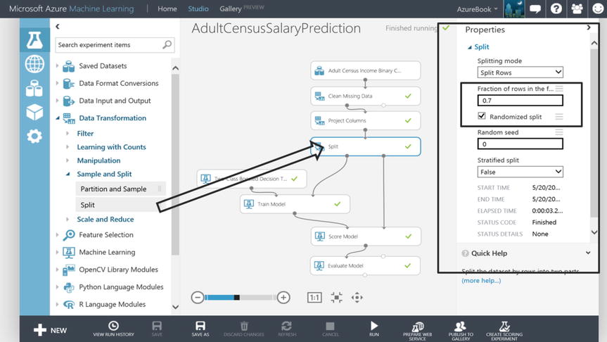
Figure 14-18. Machine Learning Split Module
The Split module’s input port is connected to the output port of the Project Columns module. The Split module’s property pane shows that 70% of the data will be sent through the first output port to train the model. The data selection to satisfy that 70% will be done randomly, as indicated by the presence of the checked box (see Figure 14-18). An experiment author will choose how much data to train the model with based on their understanding of the data. Perhaps the dataset is small and the author believes the best predictive results will come from training the model with a majority of the data. It is also very common to see a 50% split where half the data is used to train the model and the other half is used to test the model’s effectiveness at prediction. In fact, the Split module’s default property settings are preset to 50%.
An algorithm is chosen along with the Train Model module to crunch 70% of the census data. Because the dataset is classified with income as “<=50” and “>50”, it would make sense to choose a classification algorithm. Since the dataset has 2 classes this helps to further limit the algorithm selection by looking for Two-Class algorithms. To this end, the Two-Class Boosted Decision Tree module is used in the experiment. The Train Model module is used to stitch 70% of the data together with the algorithm, as illustrated in Figure 14-19.
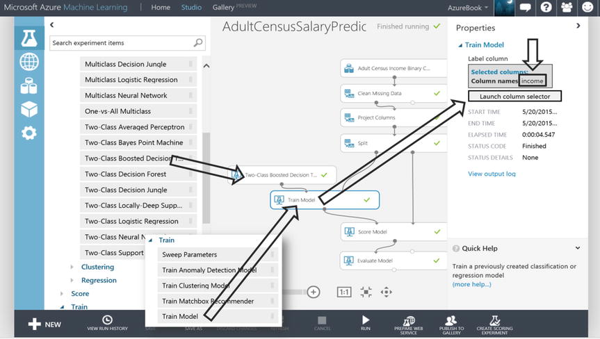
Figure 14-19. Machine Learning Train Model Module
![]() Note For any module, and particularly useful for algorithm modules, there exists a “Quick Help” link at the bottom of the property pane. Click this link for technical documentation on a given algorithm. A useful algorithm selection decision tree can be found in the following blog entry authored by Brandon Rohrer from Microsoft, https://azure.microsoft.com/en-us/documentation/articles/machine-learning-algorithm-cheat-sheet/
Note For any module, and particularly useful for algorithm modules, there exists a “Quick Help” link at the bottom of the property pane. Click this link for technical documentation on a given algorithm. A useful algorithm selection decision tree can be found in the following blog entry authored by Brandon Rohrer from Microsoft, https://azure.microsoft.com/en-us/documentation/articles/machine-learning-algorithm-cheat-sheet/
The Train Model module, illustrated in Figure 14-19, initially has no idea about what the dataset label is required for training the Two-Class Boosted Decision Tree algorithm. The Launch Column selector button in the property pane for the Train Model module is used to choose column income as the label whose contents will be analyzed to train the model. The goal is to effectively predict the label classes “<=50” and “>50”.
Once income is selected as the label column, the Two-Class Boosted Decision Tree algorithm module will use the other columns in the data flow as features (education, age, marital-status, etc.) as it teaches itself to predict “>50” and “<=50”.
Score and Evaluate
After the model is trained, the results need to be evaluated. To test the model, new instances (rows) of individuals need to be introduced and scored. These will be the individuals representing 30% of the dataset based on the Split module configured earlier. Scoring the new individuals is essentially asking the trained model to only look at the individual’s features and score them with the likelihood of “>50”. This is akin to telling the trained model “given these individual’s features, like age, education, gender and the like, calculate the probability that they will earn more than $50,000” In the experiment, the output port of the Train Model module coupled with the output port on the right side (30% of data) of the Split module are connected to the respective input ports of the Score Model module, Figure 14-20.
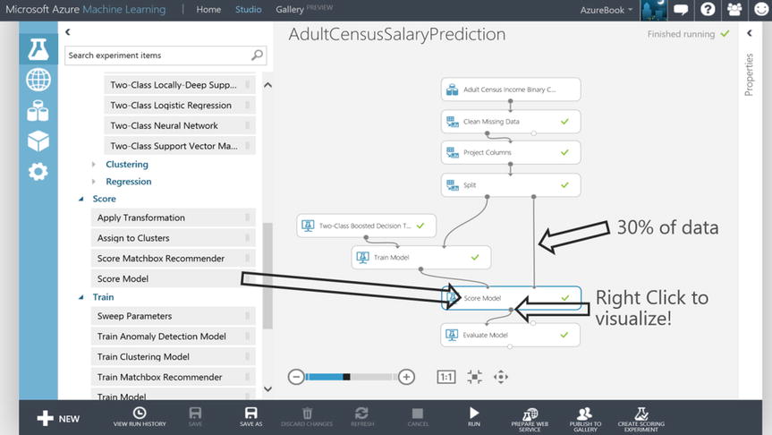
Figure 14-20. Machine Learning Score Model Module
After the “Score Model” module has RUN, two additional columns are added to the dataset that flows out of the Score Model module output port. The two columns show the probability of the likelihood that the individual will be “>50” as well as the predicted label itself (“<=50” or “>50”). This means that if a given individual is scored as 51.4568% probability, then the scored label would be “>50”. Alternatively, if the individual was scored as 49.0934% probability that they would be “>50”, then the scored label in this case would be “<=50”. Another way to read the second example is that the individual has a 50.9066% (100 - 49.0934) probability of being “<=50”. This is a little confusing, but since the focus is on whether the individual will make “>50”, the scoring is relative to that class.
The “>50” is the Positive classification. If the algorithm indicates that there is a 50% chance (or better) that a given individual is “>50”, and after peeking at the training data it finds that “>50” is the actual value, then that prediction outcome is a True Positive. Conversely, if the actual value is “<=50” then that would be a False Positive. It works the other way as well. If the algorithm indicates that there is a less than 50% chance the individual is “>50”, then that is the Negative case and it would have the scored label “<=50”. If the actual value for this individual in the training data was “>50”, then a prediction of “<=50” would be a False Negative. If the actual value is “<=50”, then a prediction of “<=50” is a True Negative.
To visualize the Score Model module dataset, the output port can be clicked followed by the selection of Visualize. Using arrow keys to scroll to the right within the viewer, 2 new columns are found: Scored Probability and Scored Label, see Figure 14-21. Notice in Figure 14-21 the column income has the actual income (“<=50”, “>50”) of the individuals. The Scored Labels column is what the Two-Class Boosted Decision Tree predicts for this individual after the model is trained. In some cases the actual value (in the income label column) is different than the algorithm’s predicted Scored Labels column. An example of this is captured in Figure 14-21. The greyed rectangles illustrate False Negatives.
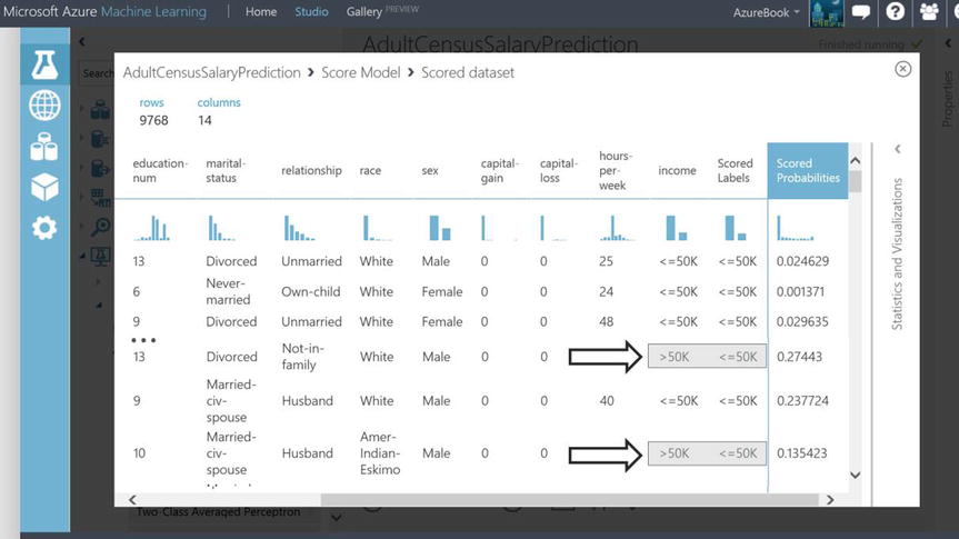
Figure 14-21. Machine Learning Score Model Dataset
With all of the True Positives (TP), False Positives (FP), True Negatives (TN) and False Negatives (FN) it is easy to see that tallying them up as they relate to the total count of individuals scored, could provide some insight into the effectiveness of the trained model.
For example, assume 10,000 individuals were scored and it was known that 100 of them had income “>50”. If the algorithm scored 80 of those individuals correctly (it predicted 80 out the 100) and the algorithm’s false positive calculation of “>50” was relatively high, say 35, then this would only be a somewhat precise model.
A common way to represent the counts of TP, FP, TN and FN is through a confusion matrix. A confusion matrix is a way to visualize the performance of the predictions, showing both what was predicted and what the actual value was during the scoring process. Figure 14-22 is a confusion matrix for the hypothetical 10,000-instance example.
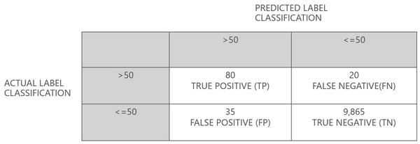
Figure 14-22. Machine Learning Confusion Matrix
To calculate the overall accuracy of the hypothetical 10,000 individuals scored with the trained model, the calculation below is performed. Accuracy is to say “Of the entire data population, how good was the model at predicting either <=50 or >50?”
- Accuracy = (TP+TN)/(TP+FP+TN+FN)
- Accuracy = (80+9865)/(80+35+9865+20) = 99%
The following formula calculates the precision of the model (looking at true positive ratio). This calculation says “When the model predicts >50, how often is it right?”
- Precision = TP/(TP+FP)
- Precision = 80/(80+35) = 70%
Another performance metric is recall. Which is to say “With the total population of actual >50, how good is the model at predicting them”:
- Recall = TP/(TP+FN)
- Recall = 80/(80+20) = 80%
In the example, when the model predicts the individual to have an income greater than $50,000 (>50), it is right 70% of the time. In other words, a prediction of “>50” comes with a 30% chance of representing a False Positive (actual of <=50). Generally speaking, whether the model predicts either “<=50” or “>50” the overall prediction accuracy is near perfect (99%). This is not hard to believe as the vast majority of the individuals in the example have actuals of “<=50” and with a TN rate that is in line with the actual count, it comes with little surprise that the accuracy is so high. The model does leave a few individuals with income greater than $50,000 left behind as false negatives, predicted as making less than or equal to $50,000. But, the recall is 80%, meaning when “>50” is predicted the majority of actual “>50” are being represented.
The confusion matrix is a powerful tool to visualize the performance of the Two-Class Boosted Decision Tree algorithm module. In ML Studio not only is it possible to view the model’s confusion matrix, but a line chart is also provided where on the X axis the false positive rate is plotted and on the Y axis the true positive rate is plotted. The module that provides these performance metrics and visualizations is the Evaluate Model module as shown in Figure 14-23.
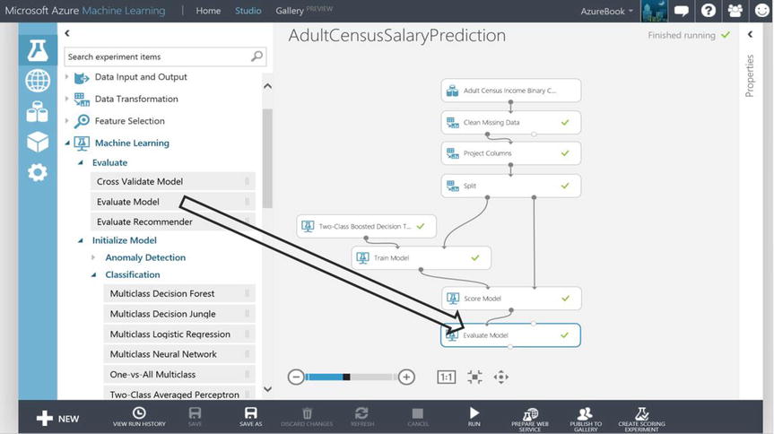
Figure 14-23. Machine Learning Evaluate Model Module
The Evaluate Model module has two input ports. Both are not required to be connected, but an interesting aspect of this module is that it can be used to compare the performance of two different scored datasets, perhaps the scored datasets came from different trained models that used different classification algorithms. In the AdultCensusSalaryPrediction experiment, only the first input port is connected to the previously scored dataset. The output of the Evaluate Model module is visualized by clicking its output port and then clicking Visualize. The results are shown in Figure 14-24.

Figure 14-24. Machine Learning Evaluate Model Visualization
The curve is called an ROC curve. A model that performs well has a larger area under the curve (AUC) than above the curve. The closer the curve gets to the line diagonally cutting across the grid, the greater the chance that a random guess is just as good as the model. The confusion matrix is in the screen shot overlay as illustrated in Figure 14-24.
By dragging the Threshold slider to the right, the precision calculation typically improves. The threshold slider is a convenient way to assess precision as the probability of “>50” increases based on the value of the slider. The threshold slider calculates precision based on the count of true positives and false positives where “>50” is predicted at or above the percentage represented by the slider. If the slider was moved to .8, then the precision calculation would be based on the count of TP and FP where the likelihood of “>50” is 80% or higher. In this case, TP is 964 and FP is 120. The precision would then be 964/ (964+120) = .889 as illustrated in Figure 14-24.
The trained model in the experiment AdultCensusSalaryPrediction has accuracy, precision, and recall prediction results of 99%, 70%, and 80% respectively. These results are significantly better than a 50% random guess as to whether an individual will be “<=50” or “>50”. Both from a precision and an accuracy perspective the evaluation of the model results in predictions that most organizations would be comfortable taking action on. The nature of a business problem and the benefit of the prediction coupled with the cost and risk of taking action on a false positive need to be weighed to determine if a model is considered viable. If the AdultCensusSalaryPrediction experiment and its trained model were used for shaping policy around fair wages or refining a marketing strategy, then it would be a sound experiment to operationalize.
Quick Hands-On Operationalizing an Experiment
If the experiment AdultCensusSalaryPrediction evaluates well and has been ascertained to effectively predict income, it would make sense to operationalize the experiment if appropriate business justification supports the effort.
An example of a business justification might include a marketing firm that wants to run the experiment against demographic data they have collected so that they can identify prospective customers that make more than $50,000 dollars. This kind of information could drive a marketing strategy. Another example could be a government entity that wants to ensure fair wages. In this case the experiment might be ran against new individual’s data where their features could be tweaked (maybe change the feature Sex from “Male” to “Female”) to see if the same income is predicted. If a disparity is found, then decisions might be made to correct a potential bias.
To prepare the Azure Machine Learning experiment to be operational, first the model must be saved as a self-contained unit of work encapsulating the algorithm, what features it expects, what label and associated classes are being predicted and so on.
The goal of this exercise is to create a web service that can be invoked from an application, from Excel, or from any system that can execute and report results for a web service.
In the marketing example, perhaps that organization wants to process all new customers that have entered their demographic data matching the features for the AdultCensusSalaryPrediction experiment. The organization’s developer would have designed a weekly batch process that invokes a web service calling the experiment with the feature data entered by customers and getting predicted salary in return. The predicted salary results will establish which marketing campaign to assign to the each new customer.
The following steps walk through the exercise of configuring a web service for the AdultCensusSalaryPrediction experiment:
- In the experiment AdultCensusSalaryPrediction, click the output port of the Train Model module and then click Save as Trained Model, as illustrated in Figure 14-25. Give the saved trained model a name, call it “Individuals50K”.
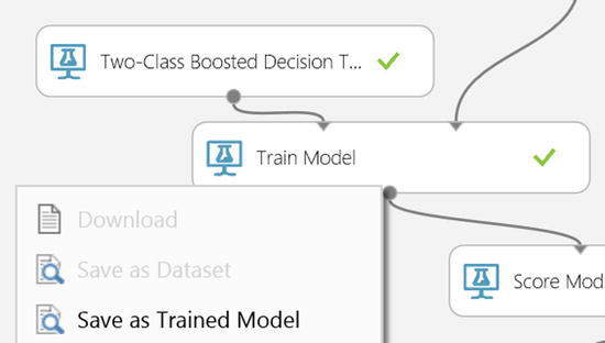
Figure 14-25. Saving Machine Learning Train Models
Next step is to copy the experiment AdultCensusSalaryPrediction to another experiment and name it so it can be recognized as an operational experiment. Perhaps precede the name with “prod” for production:
- When the canvas is displaying the experiment AdultCensusSalaryPrediction, click Save As at the bottom of the screen and name the new experiment prodAdultCensusSalaryPrediction.
The following steps prepare the experiment prodAdultCensusSalaryPrediction to only contain what is necessary for production:
- Right click and delete (or highlight and press del-key) the modules: Split, Two-Class Boosted Decision Tree, Train Model, and Evaluate Model.
- In the left hand pane modules list and under the Trained Models heading, drag and drop the trained model you saved (Individuals50K) onto the canvas and connect the ports as illustrated in Figure 14-26.
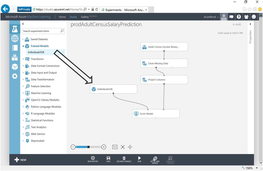
Figure 14-26. Copying Machine Learning Experiments
- Click on SET UP WEB SERVICE at the bottom of the canvas.
- Click on RUN at the bottom of the canvas.
- Click on DEPLOY WEB SERVICE at the bottom of the canvas. You are now presented with the screen in Figure 14-27.
Note There is tremendous power with the ease at which a web service can be created from an Azure Machine Learning experiment. When in the web service dashboard page as illustrated in Figure 14-27 and clicking on REQUEST/RESPONSE, all of the API Helper code is provided allowing the developer to easily deploy a web service that will execute the experiment prodAdultCensusSalaryPrediction.
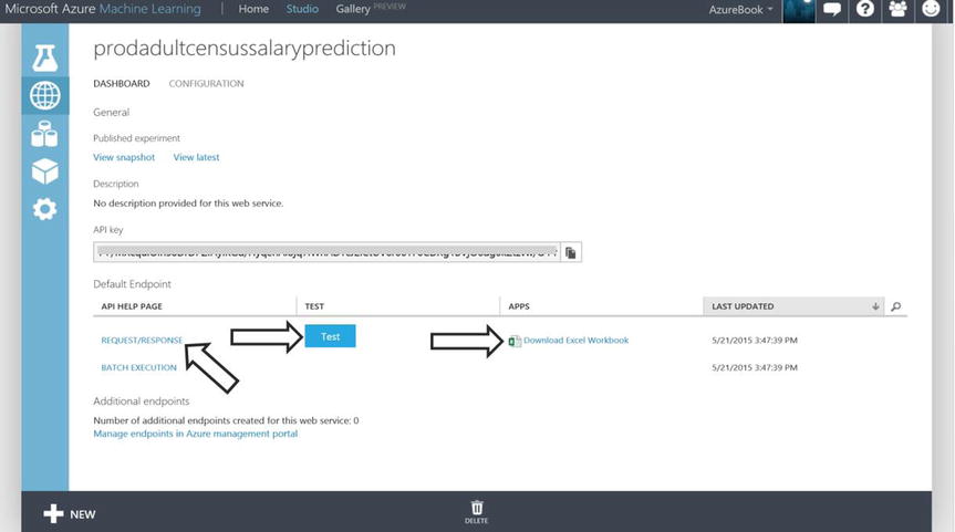
Figure 14-27. Publishing a Machine Learning Experiment as a Web Service
- Test the web service by clicking on Test as shown in Figure 14-27 above. You are now presented with many of the features from the original census dataset as seen in Figure 14-28.
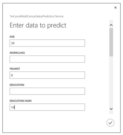
Figure 14-28. Web Service “Test” Dialog with Features
- Enter the following feature values: age=39, education-num=14, married-status=Married-civ-spouse, relationship=Wife, race=White, sex=Female, hours-per-week=45, Figure 14-28.
Note By populating the Test dialog fields with categorical values relevant for the trained model, you will see some valid scored results returned. When entering the data, you ignore income as that is what the model is predicting.
- Click on the check mark in the lower right corner of the Test dialog. You will see the web service results returned with the last element being the Scored Probability equal to “.88316…” and Scored Labels equal “>50K”. Meaning, for this individual, the trained model predicts an 88% likelihood their income is greater than $50,000, Figure 14-29. You just invoked a web service that ran your experiment prodAdultCensusSalaryPrediction!
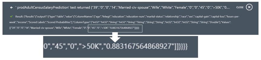
Figure 14-29. Web Service Completion String
The Azure Machine Learning web service dashboard illustrated in Figure 14-27 allows the user to download a sample Excel workbook that has been pre-wired with macros enabling it to execute the web service.
- Click Download Excel Workbook and open the Excel Workbook, see Figure 14-30.
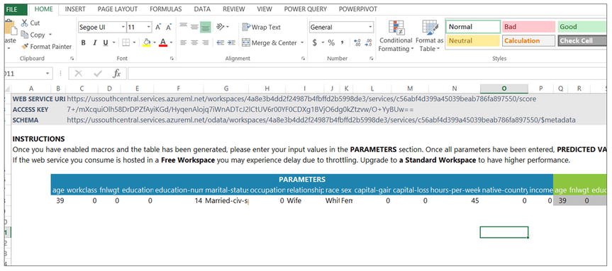
Figure 14-30. Excel Workbook from Azure Machine Learning Studio
- Enable the content to allow macros. This will be a prompt Excel displays to the user. In Figure 14-30 the workbook has already been enabled.
- Enter: age=39, education-num=14, married-status=Married-civ-spouse, relationship=Wife, race=White, sex=Female, hours-per-week=45 as seen in Figure 14-30.
- Look at the scores on the right hand side of the matrix in Excel, you may need to scroll to the right. It should show around 88% as illustrated in Figure 14-31.
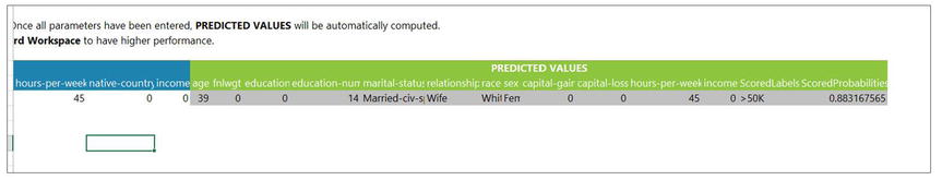
Figure 14-31. Excel Workbook Predictions
- Now play around with the individual’s features and categories to see what the web service experiment produces.
The ramifications of this simple exercise are profound. A business could publish the web service to the Azure Market Place, provide their business information and collect 10 cents every time someone executes the Azure Machine Learning web service to predict income.
The web service could be included in an organization’s operational internal ETL (Extract Transform Load) processes, scoring data as it flows through a business data transform.
![]() Note The web service could also have been deployed with neither inputs nor outputs. Consider a scenario where the experiment author dropped the Reader module onto the experiment canvas, configured it to read an Azure SQL Database staging table where the new individuals to be scored reside. The experiment processes what is in the stage table and writes the scored results to an Azure SQL Database reporting table that is accessed through the Writer module that was also dropped onto the canvas. The Writer module’s input port would be connected to the output port of the Score Model module. In this hypothetical case, after the web service is created from the experiment and then invoked, it would simply read from a stage table and write to a report table. Using this strategy, the DBA has their role in setting up the stage and reporting tables in Azure SQL Database. The analyst simply reports against the report table and the data scientist did all of the Azure Machine Learning work. This scenario speaks to the ability to bring IT and business roles into a complete data analytics lifecycle, where any given person need not know what the others did, they each have their place and the whole of their efforts is much greater than the sum of their parts. Play this video to see such a scenario in action, https://youtu.be/ABsOnmOzIUI
Note The web service could also have been deployed with neither inputs nor outputs. Consider a scenario where the experiment author dropped the Reader module onto the experiment canvas, configured it to read an Azure SQL Database staging table where the new individuals to be scored reside. The experiment processes what is in the stage table and writes the scored results to an Azure SQL Database reporting table that is accessed through the Writer module that was also dropped onto the canvas. The Writer module’s input port would be connected to the output port of the Score Model module. In this hypothetical case, after the web service is created from the experiment and then invoked, it would simply read from a stage table and write to a report table. Using this strategy, the DBA has their role in setting up the stage and reporting tables in Azure SQL Database. The analyst simply reports against the report table and the data scientist did all of the Azure Machine Learning work. This scenario speaks to the ability to bring IT and business roles into a complete data analytics lifecycle, where any given person need not know what the others did, they each have their place and the whole of their efforts is much greater than the sum of their parts. Play this video to see such a scenario in action, https://youtu.be/ABsOnmOzIUI
Summary
With the ease, power, and flexibility of authoring experiments in ML Studio, coupled with the “click and go” web service integration of Azure Machine Learning, you have a cloud platform that is approachable to a broad audience of IT professionals, data enthusiasts, as well as traditional data scientists.