1
Three-dimensional Modeling
This chapter looks at the three-dimensional modeling of a solid (non-articulated) robot. Such modeling is used to represent airplanes, quadcopters, submarines, and so on. Through this modeling we will introduce a number of fundamental concepts in robotics such as state representation, rotation matrices and Euler angles. The robots, whether mobile, manipulator or articulated, can generally be put into a state representation form:
where x is the state vector, u the input vector and y the vector of measurements [JAU 05]. We will call modeling the step which consists of finding a more or less accurate state representation of the robot. In general, constant parameters may appear in the state equations (such as the mass and the moment of inertia of a body, viscosity, etc.). In such cases, an identification step might prove to be necessary. We will assume that all of the parameters are known. Of course, there is no systematic methodology that can be applied for modeling a mobile robot. The aim of this chapter is to present the tools which allow us to reach a state representation of three-dimensional solid robots in order for the reader to acquire a certain experience which will be helpful when modeling his/her own robots. This modeling will also allow us to recall a number of important concepts in Euclidean geometry, which are fundamental in mobile robotics. This chapter begins by recalling a number of important concepts in kinematics which will be useful for the modeling.
1.1. Rotation matrices
For three-dimensional modeling, it is essential to have a good understanding of the concepts related to rotation matrices, which are recalled in this section. It is by using this tool that we will perform our coordinate system transformations and position our objects in space.
1.1.1. Definition
Let us recall that the jth column of the matrix of a linear application of ℝn → ℝn represents the image of the jth vector ej of the standard basis (see Figure 1.1). Thus, the expression of a rotation matrix of angle θ in the plane ℝ2 is given by:

Figure 1.1. Rotation of angle θ in a plane
Concerning rotations in the space ℝ3 (see Figure 1.2), it is important to specify the axis of rotation. We distinguish three main rotations: the rotation around the Ox axis, around the Oy axis and around the Oz axis.

Figure 1.2. Rotations in ℝ3 following various viewing angles
The associated matrices are respectively given by:

Let us recall the formal definition of a rotation. A rotation is a linear application which is an isometry (i.e. it preserves the scalar product) and is direct (it does not change the orientation in space).
THEOREM.– A matrix R is a rotation matrix if and only if:
PROOF.– The scalar product is preserved by R if, for any u and v in ℝn, we have:
Therefore RTR = I. The symmetries relative to a plane, as well as all the other improper isometries (isometries that change the orientation of space, such as a mirror), also verify the property RT·R = I. The condition det R = 1 allows us to be limited to the isometries which are direct. ■
1.1.2. Lie group
The set of rotation matrices of ℝn forms a group with respect to the multiplication. It is referred to as a special orthogonal group (special because det R =1, orthogonal because RT·R = I) and denoted by SO(n). It is trivial to check that (SO(n), ·) is a group where I is the neutral element. Moreover, the multiplication and the inversion are both smooth. This makes SO(n) a Lie group which is a manifold of the set of matrices ℝn×n.
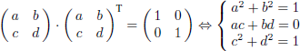
The set ℝn×n of n × n-matrices is of dimension n2. Since the matrix RT · R is always symmetric, the matrix equation RT · R = I can be decomposed into ![]() independent scalar equations. For instance, for n = 2, we have
independent scalar equations. For instance, for n = 2, we have ![]() scalar equations:
scalar equations:
As a consequence, the set SO(n) forms a manifold of dimension ![]() .
.
- – for n = 1, we get d = 0. The set SO (1) is a singleton which contains a single rotation matrix: R =1;
- – for n = 2, we get d =1. We need a unique parameter (or angle) to represent the rotations of SO(2);
- – for n = 3, we get d = 3. We need three parameters (or angles) to represent SO (3).
1.1.3. Lie algebra
An algebra is an algebraic structure ![]() over a body
over a body ![]() , if (i)
, if (i) ![]() is a vector space over
is a vector space over ![]() ; (ii) the multiplication rule × of
; (ii) the multiplication rule × of ![]() is left- and right-distributive with respect to +; and (iii) for all α,
is left- and right-distributive with respect to +; and (iii) for all α, ![]() , and for all x,
, and for all x, ![]() , α·x × β ·y and (αβ) · (x × y). Notice that in general, an algebra is non-commutative (x × y ≠ y × x) and non-associative ((x × y) × z ≠ x × (y × z)). A Lie algebra
, α·x × β ·y and (αβ) · (x × y). Notice that in general, an algebra is non-commutative (x × y ≠ y × x) and non-associative ((x × y) × z ≠ x × (y × z)). A Lie algebra ![]() is a non-commutative and non-associative algebra in which multiplication, denoted by a so-called Lie bracket, verifies that (i) [·, ·] is bilinear, i.e. linear with respect to each variable; (ii) [x, y] = − [y, x] (antisymmetry) and (iii) [x, [y, z]] + [y, [z, x]] + [z, [x, y]] = 0 (Jacobi relation).
is a non-commutative and non-associative algebra in which multiplication, denoted by a so-called Lie bracket, verifies that (i) [·, ·] is bilinear, i.e. linear with respect to each variable; (ii) [x, y] = − [y, x] (antisymmetry) and (iii) [x, [y, z]] + [y, [z, x]] + [z, [x, y]] = 0 (Jacobi relation).
For Lie groups, we can define the associated Lie algebras. Lie algebras allow us to consider infinitesimal motions around a given element (i.e. a rotation matrix) in order to use derivatives or differential methods.
Consider the rotation matrix I of SO(n) corresponding to the identity. If we move I by adding a small matrix, say A · dt of ℝn×n, we generally do not obtain a rotation matrix. We are interested in matrices A such that I + A · dt ∈ SO(n). We have
i.e. A · dt + AT · dt = 0 + o (dt). Therefore, A should be skew-symmetric. This means that we are able to move in SO(n) around I by adding infinitesimal skew-symmetric matrices A · dt that are not elements of SO(n). This corresponds to a new operation in SO(n) which is not the multiplication that we already had. Formally, we define the Lie algebra associated with SO(n) as follows:
and it corresponds to the skew-symmetric matrices of ℝn×n.
If we now want to move around any matrix R of SO(n), we generate a rotation matrix around I and we transport it to R. We get R (I + A · dt) where A is skew-symmetric. This means that we add to R the matrix R · A · dt.
In robotics, Lie groups are often used to describe transformations (such as translations or rotations). The Lie algebra corresponds to velocities or equivalently to infinitesimal transformations. Lie group theory is useful, but requires some non-trivial mathematical backgrounds that are beyond the scope of this book. We will try to focus on SO (3) or use more classical tools such as Euler angles and rotation vectors, which are probably less general but are sufficient for control purposes.
1.1.4. Rotation vector
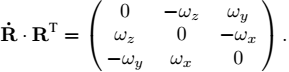
If R is a rotation matrix depending on time t, by differentiating the relation RRT = I, we get
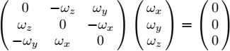
Thus, the matrix ![]() is a skew-symmetric matrix (i.e. it satisfies AT = −A and therefore its diagonal contains only zeroes, and for each element of A, we have (aij = −aji). We may therefore write, in the case where R is of dimension 3 × 3:
is a skew-symmetric matrix (i.e. it satisfies AT = −A and therefore its diagonal contains only zeroes, and for each element of A, we have (aij = −aji). We may therefore write, in the case where R is of dimension 3 × 3:
The vector ω = (ωx, ωy, ωz) is called the rotation vector associated with the pair ![]() . It must be noted that
. It must be noted that ![]() is not a matrix with good properties (such as for instance the fact of being skew-symmetric). On the other hand, the matrix
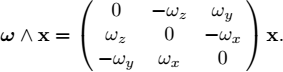
is not a matrix with good properties (such as for instance the fact of being skew-symmetric). On the other hand, the matrix ![]() has the structure of equation [1.1] since it allows positioning within the coordinate system in which the rotation is performed, and this is due to the change of basis performed by RT. We will define the cross product between two vectors ω and x ∈ ℝ3 as follows:
has the structure of equation [1.1] since it allows positioning within the coordinate system in which the rotation is performed, and this is due to the change of basis performed by RT. We will define the cross product between two vectors ω and x ∈ ℝ3 as follows:

1.1.5. Adjoint
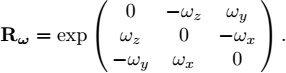
For each vector ω = (ωx, ωy, ωz), we may adjoin the skew-symmetric matrix:

which can be interpreted as the matrix associated with a cross product by the vector ω. The matrix Ad (ω) is also written ω∧.
PROPOSITION.– If R(t) is a rotation matrix that depends on time, its rotation vector is given by:
PROOF.– This relation is a direct consequence of equation [1.1]. ■
PROPOSITION.– If R is a rotation matrix in ℝ3 and if a is a vector of ℝ3, we have:
which can also be written as
PROOF.– Let x be a vector of ℝ3. We have:
PROPOSITION.– (Duality) We have:
This relation expresses the fact that the matrix ![]() is associated with the rotation vector ω, associated with R (t) but expressed in the coordinate system associated with R, whereas
is associated with the rotation vector ω, associated with R (t) but expressed in the coordinate system associated with R, whereas ![]() is associated with the same vector, but this time expressed in the coordinate system of the standard basis.
is associated with the same vector, but this time expressed in the coordinate system of the standard basis.
PROOF.– We have:
1.1.6. Rodrigues rotation formulas
Matrix exponential. Given a square matrix M of dimension n, its exponential can be defined as:
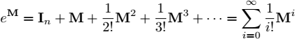
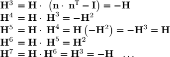
where In is the identity matrix of dimension n. It is clear that eM is of the same dimension as M. Here are some of the important properties concerning the exponentials of matrices. If 0n is the zero matrix of n × n and if M and N are two matrices n × n, then:

Matrix logarithm. Given a matrix M, the matrix L is said to be a matrix logarithm of M if eL = M. As for complex numbers, the exponential function is not a one-to-one function and matrices may have more than one logarithm. Using power series, we define the logarithm of a square matrix as
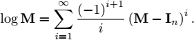
The sum is convergent if M is close to identity.
Rodrigues formulas. A rotation matrix R has an axis represented by a unit vector n and an angle α with respect to this axis. From n and α we can also generate the matrix R. The link R ↔ (n, α) is made by the following Rodrigues formulas
The first equation (i) will be shown in exercise 1.4 and (ii) is the reciprocal of (i). In these formulas, αn∧ is a notation to represent the matrix Ad (αn). As will be shown in exercise 1.4, R = eαn∧ is a rotation matrix and n is an eigenvector associated with the eigenvalue 1 of R.
Axis and angle of a rotation matrix. Given a rotation matrix R, the axis can be represented by normalized eigenvector n associated with the eigenvalue λ = 1 (two of them can be found, but we need one). To compute α and n, we may use the relation αn = log R, which works well if R is close to identity. In the general case, it is more suitable to use the following proposition.
PROPOSITION.– Given a rotation matrix R, we have R = eαn∧ where
PROOF.– Take a rotation matrix R with eigenvalues 1, λ1, λ2 and eigenvectors n, v1, v2. Consider the generalized polynomial f (x) = x − x−1, where x is the indeterminate. From the correspondence theorem of eigenvalues/vectors, the eigenvalues of f (R) = R − R−1 = R − RT are f (1) = 0, f (λ2), f (λ3) and the eigenvectors are still n, v1, v2. Since f (R) is skew symmetric and f (R) · n = 0, we have f (R) ∝ Adn. Thus, the vector Ad−1 (R − RT) is an eigenvector of R associated with the eigenvalue 1. It provides us the axis of R. To find the angle α, we use the property that the trace of a matrix is similarity-invariant, which means that for any invertible matrix P, we have tr(R) = tr(P−1 · R · P). Take P as the rotation matrix with transforms R into a rotation along the first axis. We get
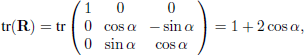
which provides us with the angle of the rotation. Exercise 1.5 provides a geometrical proof of this proposition. ■
1.1.7. Coordinate system change
Let ![]() and
and ![]() be two coordinate systems and let u be a vector of ℝ3 (refer to Figure 1.3). We have the following relation:
be two coordinate systems and let u be a vector of ℝ3 (refer to Figure 1.3). We have the following relation:
where (x0, y0, z0) and (x1, y1, z1) are the coordinates of u in ![]() and
and ![]() , respectively.
, respectively.
Thus, for any vector v we have:
By taking respectively v = i0, j0, k0, we obtain the following three relations:
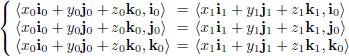

Figure 1.3. Changing the coordinate system  to the system
However, since the basis (i0, j0, k0) of ![]() is orthonormal, 〈i0, i0〉 = (j0, j0) = 〈k0, k0〉 = 1 and 〈i0, j0〉 = 〈j0, k0〉 = 〈i0, k0〉 = 0. Thus, these three relations become:
is orthonormal, 〈i0, i0〉 = (j0, j0) = 〈k0, k0〉 = 1 and 〈i0, j0〉 = 〈j0, k0〉 = 〈i0, k0〉 = 0. Thus, these three relations become:

or in matrix form:

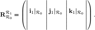
We can see a rotation matrix ![]() whose columns are the coordinates of i1, j1, k1 expressed in the absolute system
whose columns are the coordinates of i1, j1, k1 expressed in the absolute system ![]() . Thus,
. Thus,
This matrix depends on time and links the frame![]() to
to ![]() . The matrix
. The matrix ![]() is often referred to as a direction cosine matrix since its components involve the direction cosines of the basis vectors of the two coordinate systems. Likewise, if we had several systems
is often referred to as a direction cosine matrix since its components involve the direction cosines of the basis vectors of the two coordinate systems. Likewise, if we had several systems ![]() (see Figure 1.4), we would have:
(see Figure 1.4), we would have:
Dead Reckoning. Let us consider the situation of a robot moving in a three-dimensional environment. Let us call ![]() its reference frame (for example, the frame of the robot at an initial time). The position of the robot is represented by the vector p(t) expressed in
its reference frame (for example, the frame of the robot at an initial time). The position of the robot is represented by the vector p(t) expressed in ![]() and its attitude (i.e. its orientation) by the rotation matrix R(t) which represents the coordinates of the vectors i1, j1, k1 of the coordinate system
and its attitude (i.e. its orientation) by the rotation matrix R(t) which represents the coordinates of the vectors i1, j1, k1 of the coordinate system ![]() of the robot expressed in the coordinate system
of the robot expressed in the coordinate system ![]() , at time t. It follows that:
, at time t. It follows that:


Figure 1.4. Composition of rotations
This matrix can be returned by a precise attitude unit positioned on the robot. If the robot is also equipped with a Doppler Velocity Log (or DVL) which provides it with its speed vector vr relative to the ground or the seabed, expressed in the coordinate system ![]() of the robot, then the speed vector v of the robot satisfies:
of the robot, then the speed vector v of the robot satisfies:

or equivalently:
Dead reckoning consists of integrating this state equation from the knowledge of R(t) and vr (t).
1.2. Euler angles
1.2.1. Definition
In related literature, the angles proposed by Euler in 1770 to represent the orientation of solid bodies in space are not uniquely defined. We mainly distinguish between the roll-yaw-roll, roll-pitch-roll and roll-pitch-yaw formulations. It is the latter that we will choose since it is imposed in the mobile robotics language. Within this roll-pitch-yaw formulation, the Euler angles are sometimes referred to as Cardan angles. Any rotation matrix of ℝ3 can be expressed in the form of the product of three matrices as follows:

or, in developed form:
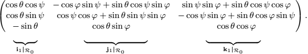
The angles φ, θ, ψ are the Euler angles and are respectively called the bank, the elevation and the heading. The terms roll, pitch, yaw are often employed, although they correspond, respectively, to variations of bank, elevation and heading.
Gimbal lock. When ![]() (the same effect happens as soon as cos θ = 0), we have
(the same effect happens as soon as cos θ = 0), we have

and thus,
This corresponds to a singularity which tells us that when ![]() , we cannot move on the manifold of rotation matrices SO(3) in all directions using the Euler angles. Equivalently, this means that some trajectories R(t) cannot be followed by Euler angles.
, we cannot move on the manifold of rotation matrices SO(3) in all directions using the Euler angles. Equivalently, this means that some trajectories R(t) cannot be followed by Euler angles.
Rotation matrix to Euler angles. Given a rotation matrix R, we can easily find the three Euler angles by solving, following equation [1.9], the equations:
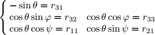
By imposing ![]() , φ ∈ [−π, π] and ψ ∈ [−π, π], we find:
, φ ∈ [−π, π] and ψ ∈ [−π, π], we find:
Here atan2 is the two-argument arctangent function defined by
1.2.2. Rotation vector of a moving Euler matrix
Let us consider a solid body moving in a coordinate system ![]() and a coordinate system
and a coordinate system ![]() attached to this body (refer to Figure 1.5). The conventions chosen here are those of the SNAME (Society of Naval and Marine Engineers). The two coordinate systems are assumed to be orthonormal. Let R(t) = R(ψ(t), θ(t), φ(t)) be the rotation matrix that links the two systems. We need to find the instantaneous rotation vector ω of the solid body relative to
attached to this body (refer to Figure 1.5). The conventions chosen here are those of the SNAME (Society of Naval and Marine Engineers). The two coordinate systems are assumed to be orthonormal. Let R(t) = R(ψ(t), θ(t), φ(t)) be the rotation matrix that links the two systems. We need to find the instantaneous rotation vector ω of the solid body relative to ![]() in function of φ, θ, ψ,
in function of φ, θ, ψ, ![]() . We have:
. We have:
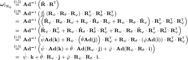
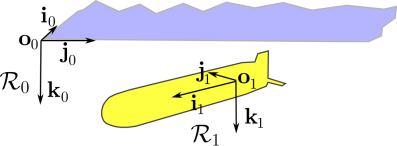
Figure 1.5. The coordinate system 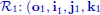 ) attached to the robot
Thus, after having calculated the quantities k, Rψ j and Rψ Rθ i in the coordinate system ![]() , we have:
, we have:
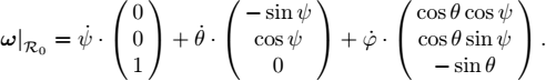
From this we get the result:
Note that this matrix is singular if and only if cos θ = 0. We will therefore take care to never have an elevation θ equal to ![]() , to avoid the gimbal lock.
, to avoid the gimbal lock.
1.3. Inertial unit
Assume that we are enclosed inside a box near to the Earth without any ability to see the environment outside. Inside the box we may perform some inertial experiments such as observing bodies translating or rotating. These experiments allow us to indirectly measure the tangential accelerations and the angular speed of the box in its own frame. The principle of an inertial unit is to estimate the pose (position and orientation) of the box from these inertial measurements only (called proprioceptive measurements), assuming that the initial pose is known.
For this purpose, we will describe the motion of our box with a kinematic model, the inputs of which are the tangential accelerations and the angular speeds, which are directly measurable in the coordinate system of the box. The state vector is composed of the vector p = (px, py, pz) that gives the coordinates of the center of the box expressed in the absolute inertial coordinate system ![]() , the three Euler angles (φ, θ, ψ) and the speed vector vr of the box expressed in its own coordinate system
, the three Euler angles (φ, θ, ψ) and the speed vector vr of the box expressed in its own coordinate system ![]() . The inputs of the system are first the acceleration
. The inputs of the system are first the acceleration ![]() of the center of the box also given in
of the center of the box also given in ![]() and second, the vector
and second, the vector ![]() corresponding to the rotation vector of the box relative to
corresponding to the rotation vector of the box relative to ![]() expressed in
expressed in ![]() . We have to express a, ω in the coordinate system of the box since these quantities are generally measured via the sensors attached on it. The first state equation is:
. We have to express a, ω in the coordinate system of the box since these quantities are generally measured via the sensors attached on it. The first state equation is:
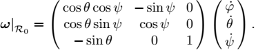
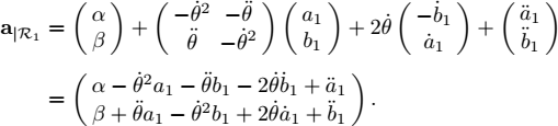
Let us differentiate this equation. We obtain:
with R = R (φ, θ, ψ). From this equation, we isolate ![]() to get
to get
which constitutes the second state equation. Figure 1.6 shows a situation where a robot has a constant speed and follows a circle. The speed vector vr is a constant whereas ar is different from zero.
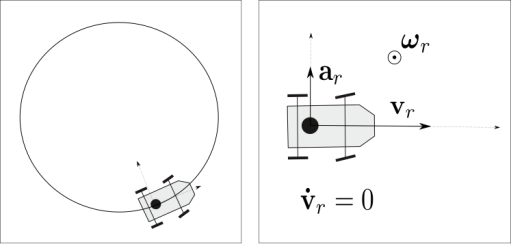
Figure 1.6. Illustration of the formula  when
when  . Left: the robot follows a circle; right: representation of the vectors in the robot frame
We also need to express ![]() in function of the state variables. From equation [1.11], the relation
in function of the state variables. From equation [1.11], the relation
becomes

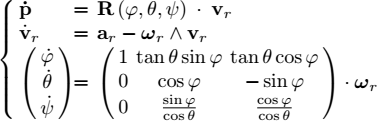
By isolating the vector ![]() in this expression, we obtain the third state equation. By bringing together the three state equations, we obtain the navigation mechanization equations [FAR 08]:
in this expression, we obtain the third state equation. By bringing together the three state equations, we obtain the navigation mechanization equations [FAR 08]:
On a horizontal plane. If we move on a horizontal plane, we have φ = θ = 0. The last equation gives us ![]() and
and ![]() . In such a case, there is a perfect correspondence between the components of ωr and the differentials of the Euler angles. There are singular cases, for instance when
. In such a case, there is a perfect correspondence between the components of ωr and the differentials of the Euler angles. There are singular cases, for instance when ![]() (this is the case when the box points upwards), in which the differentials of the Euler angles cannot be defined. Using the rotation vector is often preferred since it does not have such singularities.
(this is the case when the box points upwards), in which the differentials of the Euler angles cannot be defined. Using the rotation vector is often preferred since it does not have such singularities.
Dead reckoning. For dead reckoning (i.e. without external sensors) there are generally extremely precise laser gyrometers (around 0.001 deg/s.). These make use of the Sagnac effect (in a circular optical fiber turning around itself, the time taken by light to travel an entire round-trip depends on the path direction). Using three fibers, these gyrometers generate the vector ωr = (ωx, ωy, ωz). There are also accelerometers capable of measuring the acceleration ar with a very high degree of precision. In pure inertial mode, we determine our position by differentiating equations [1.12] only using the acceleration ar and the rotation speed ωr, both expressed in the coordinate system of the box. In the case where we are measuring the quantity vr (also expressed in the frame of the inertial unit attached to the robot) with a Doppler velocity log, we only need to integrate the first and the last of these three equations. Finally, when the robot is a correctly ballasted submarine or a terrestrial robot moving on a relatively plane ground, we know a priori that on average the bank and the elevation are equal to zero. We may therefore incorporate this information through a Kalman filter in order to limit the drift in positioning. An efficient inertial unit integrates an amalgamation of all the available information.
Inertial unit. A pure inertial unit (without hybridization and without taking into account Earth’s gravity) represents the robot by the kinematic model of Figure 1.7, which itself uses the state equations given in [1.12]. This system is written in the form ẋ = f (x, u) where u = (ar, ωr) is the vector of the measured inertial inputs (accelerations and rotation speeds viewed by an observer on the ground, but expressed in the frame of the robot) and x = (p, vr, φ, θ, ψ) is the state vector. We may use a numerical integration method such as the Euler method. This leads to replacing the differential equation ẋ = f (x, u) with the recurrence:

Figure 1.7. Navigation mechanization equations
With gravity. In the case where there exists a gravity g (p) which depends on p, the actual acceleration ar corresponds to the gravity plus the measured acceleration ![]() . In this case, the inertial unit can be described by the following state equations:
. In this case, the inertial unit can be described by the following state equations:

In this case, the inputs of the system are ![]() and ωr which are obtained by the accelerometers and the gyroscope. To integrate this state equation for localization purposes, we need to know the initial state and a gravity map g(p).
and ωr which are obtained by the accelerometers and the gyroscope. To integrate this state equation for localization purposes, we need to know the initial state and a gravity map g(p).
Using rotation matrix instead of Euler angles. From equation [1.4], we have ![]() . Thus, the state equations [1.13] can be written without any Euler angles as
. Thus, the state equations [1.13] can be written without any Euler angles as

The main advantage of this representation is that we do not have the singularity that exists in [1.13] for cos θ = 0. But instead, we have redundancies, since R of dimension 9 replaces the three Euler angles. For numerical reasons, when we integrate for a long time, the matrix R(t) may loose the property R · RT = I. To avoid this, at each iteration, a renormalization is needed, i.e. the current matrix R should be projected onto SO(3). One possibility is to use a QR factorization. A QR-decomposition of a square matrix M provides two matrices Q,R such that M = Q · R where Q is a rotation matrix and R is triangular. When M is almost a rotation matrix, R is almost diagonal and also almost a rotation, i.e. on the diagonal of R the entries are approximately ±1 and outside the entries are almost zeros. The following PYTHON code performs the projection of M on SO(3) and generates the rotation matrix M2.
Q,R = numpy.linalg.qr(M)v=diag(sign(R))M2=Q@diag(v)
1.4. Dynamic modeling
1.4.1. Principle
A robot (airplane, submarine, boat) can often be considered as a solid body whose inputs are the (tangential and angular) accelerations. These quantities are analytic functions of the forces that are at the origin of the robot’s movement. For the dynamic modeling of a submarine the reference work is Fossen’s book [FOS 02], but the related notions can also be used for other types of solid robots such as planes, boats or quadrotors. In order to obtain a dynamic model, it is sufficient to take the kinematic equations and to consider the angular and tangential accelerations caused by forces and dynamic performance. These quantities become the new inputs of our system. The link between the accelerations and the forces is done by Newton’s second law (or the fundamental principle of dynamics). Thus, for instance if f is the net force resulting from the external forces expressed in the inertial frame and m is the mass of the robot, we have
Since the speed and accelerations are generally measured by sensors embedded in the system, we generally prefer to express the speed and accelerations in the frame of the robot:
where fr is the applied forces vector expressed in the robot frame. The same type of relation, known as the Euler’s rotation equation, exists for rotations. It is given by
where τr is the applied torque and ωr is the rotation vector, both expressed in the robot frame. The inertia matrix I is attached to the robot (i.e. computed in the robot frame) and we generally choose the robot frame to make I diagonal. This relation is a consequence of Euler’s second law which states that in an inertial frame, the time derivative of the angular momentum is equal to the applied torque. In the inertial frame, this can be expressed as

1.4.2. Modeling a quadrotor
As an illustration, we consider a quadrotor (see Figure 1.8) for which we want a dynamic model. The robot has four propellers that can be tuned independently. This will allow us to control the attitude and position of the robot by changing the speeds of the motors.

Figure 1.8. Quadrotor. For a color version of this figure, see www.iste.co.uk/jaulin/robotics.zip
We distinguish the front/rear propellers (blue and black), rotating clockwise and right/left propellers (red and green), rotating counterclockwise. The value of the force generated by the ith propeller is proportional to the squared speeds of the rotors, i.e. is equal to β · ωi ·|ωi|, where β is the thrust factor. Denote by δ the drag factor and ℓ the distance between any rotor and the center of the robot. The forces and torques generated on the robot are
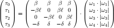
where τ0 is the total thrust generated by the rotors and τ1, τ2, τ3 are the torques generated by differences in the rotor speeds.
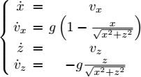
We will now show that the state equations for the quadrotor are given by
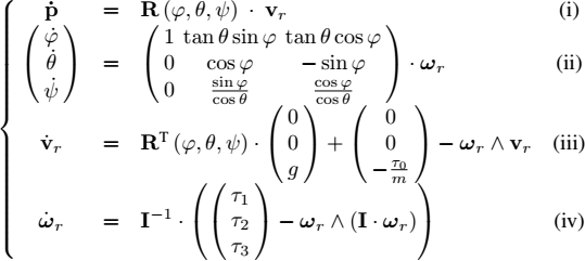
where p is the position and (φ, θ, ψ), are the Euler angles of the robot. The first three equations (i), (ii), (iii) correspond to the kinematic equations and have already been derived (see equation [1.12]). Note that in equation (iii), the acceleration ar (expressed in the robot frame) comes from Newton’s second law where the forces are the total force τ0 and the weight mg:
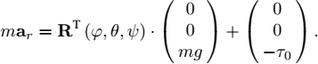
Since the gravity vector is expressed naturally in the inertial frame (contrary to the global force τ0), we have to multiply the gravity vector by the Euler rotation matrix RT (φ, θ, ψ). Equation (iv) comes from Euler’s rotation equation [1.15],
where τr = (τ1, τ2, τ3) is the torque vector.
1.5. Exercises
EXERCISE 1.1.– Properties of the adjoint matrix
Let us consider the vector ω = (ωx, ωy, ωz) and its adjoint matrix Ad (ω).
- 1) Show that the eigenvalues of Ad (ω) are {0, ||ω|| · i,−||ω|| · i}. Give an eigenvector associated with 0. Discuss.
- 2) Show that the vector Ad (ω) x = ω ∧ x is a vector perpendicular ω to and x, such that the trihedron (ω, x, to ∧ x) is direct.
- 3) Show that the norm of ω ∧ x is the surface of the parallelogram
 mediated by ω and x.
EXERCISE 1.2.– Jacobi identity
The Jacobi identity is written as:
- 1) Show that this identity is equivalent to:

where Ad (ω) is the adjoint matrix of the vector to ω ∈ ℝ3.
- 2) In the space of skew-symmetric matrices, the Lie bracket is defined as follows:

show that:

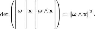
- 3) In the exercise 1.4, we will show that an infinitesimal rotation following the skew symmetric matrix A is exp
 . Consider two skew-symmetric matrices A, B and define the two infinitesimal rotation matrices

Compute a Taylor expansion of second order associated with the rotation

From this result, give an interpretation of the Lie bracket [A, B] = AB − BA.
- 4) Verify that the set (ℝ3, + , ∧, ·) forms a Lie algebra.
EXERCISE 1.3.– Varignon’s formula
Let us consider a solid body whose center of gravity remains at the origin of a Galilean coordinate system and is rotating around an axis Δ with a rotation vector of ω. Give the equation of the trajectory of a point x of the body.
EXERCISE 1.4.– Rodrigues’ formula
Let us consider a solid body whose center of gravity remains at the origin of a Galilean coordinate system and is rotating around an axis Δ. The position of a point x of the body satisfies the state equation (Varignon’s formula):
where ω is parallel to the axis of rotation Δ and ||ω|| is the rotation speed of the body (in rad.s−1).
1) show that this state equation can be written in the form:
Explain why the matrix A is often denoted by ω ∧.
2) Give the expression of the solution of the state equation.
3) Deduce from this that the expression of the rotation matrix R with angle ||ω|| around ω is given by the following formula, referred to as Rodrigues’ formula:
4) Calculate the eigenvalues of A and show that ω is the eigenvector associated with the zero eigenvalue. Discuss.
5) What are the eigenvalues of R?
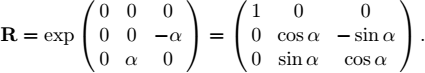
6) Using the previous questions, give the expression of a rotation around the vector ω = (1, 0, 0) of angle α.
7) Write an expression of the Euler matrix that uses Rodrigues’ formula.
EXERCISE 1.5.– Geometric approach to Rodrigues’ formula
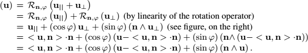
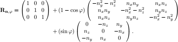
Let us consider the rotation ![]() of angle φ around the unit vector n. Let u be a vector that we will subject to this rotation. The vector u can be decomposed as follows:
of angle φ around the unit vector n. Let u be a vector that we will subject to this rotation. The vector u can be decomposed as follows:
where u∥ is collinear to n and u⊥ is in the plane P⊥ orthogonal to n (see Figure 1.9).
1) Prove Rodrigues’ formula given by:
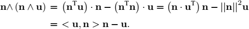
2) Using the double cross product formula a∧ (b ∧ c) = (aTc) · b − (aTb) · c, on the element n∧ (n ∧ u), show that Rodrigues’ formula can also been written as:
Deduce from this that the matrix associated with the linear operator ![]() is written as:
is written as:


Figure 1.9. Rotation Of the vector u around the vector n; Left: perspective view; right: view from above
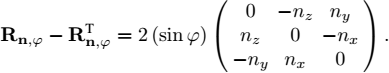
3) Conversely, we are given a rotation matrix Rn,φ for which we wish to find the axis of rotation n and the angle of rotation φ. Compute the trace tr (Rn,φ) and ![]() and use it to obtain n and φ in function of Rn,φ. For a geometric illustration, see Figure 1.10.
and use it to obtain n and φ in function of Rn,φ. For a geometric illustration, see Figure 1.10.

Figure 1.10. Left: a view of the rotation of angle φ around n; right: a visualization of the section corresponding to the Rodrigues rhombus
4) Deduce a method to find a interpolation trajectory matrix R(t) between two rotation matrices Ra, Rb such that R(0) = Ra and R(1) = Rb.
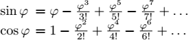
5) Using a Maclaurin series development of sinφ and cosφ, show that:
which sometimes written as:
EXERCISE 1.6.– Quaternions
Quaternions, discovered by W.R. Hamilton, are also used to represent a rotation in a three-dimensional space (see, e.g. [COR 11]). A quaternion ![]() is an extension of the complex number. It corresponds to a scalar s plus a vector v of ℝ3. We use the following equivalent notations:
is an extension of the complex number. It corresponds to a scalar s plus a vector v of ℝ3. We use the following equivalent notations:
where
1) From these relations, fill the following multiplication table:
| · | 1 | i | j | k |
| 1 | 1 | i | j | k |
| i | i | ? | ? | ? |
| j | j | ? | ? | ? |
| k | k | ? | ? | ? |
2) A unit-quaternion ![]() is a quaternion with a unit magnitude:
is a quaternion with a unit magnitude:
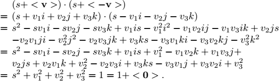
Consider the rotation obtained by a rotation around the unit vector v with an angle θ. From the Rodrigues formula, we know that the corresponding rotation matrix is exp(θ · v∧). To this rotation, we associate the quaternion:
Check that this quaternion has a unit magnitude.
3) Show that the quaternion ![]() and its opposite
and its opposite ![]() both correspond to the same rotation in ℝ3.
both correspond to the same rotation in ℝ3.
4) Assuming that the composition of rotations corresponds to a multiplication of quaternions, show that
5) We consider the Euler rotation matrix with ![]() . It corresponds to a rotation around the unit vector v with an angle α. Give the values of v and α using three methods: the geometrical method (using hands only), the matrices and the quaternions.
. It corresponds to a rotation around the unit vector v with an angle α. Give the values of v and α using three methods: the geometrical method (using hands only), the matrices and the quaternions.
EXERCISE 1.7.– Schuler pendulum
One of the fundamental components of an inertial unit is the inclinometer. This sensor gives the vertical direction. Traditionally, we use a pendulum (or a plumb line) for this. However, when we are moving, due to the accelerations the pendulum starts to oscillate and it can no longer be used to measure the vertical direction. Here, we are interested in designing a pendulum for which any horizontal acceleration does not lead to oscillations. Let us consider a pendulum with two masses m at each end, situated at a distance ℓ1 and ℓ2 from the axis of rotation of the rod (see Figure 1.11). The axis moves over the surface of the Earth. We assume that ℓ1 and ℓ2 are small in comparison to Earth’s radius r.

Figure 1.11. Inclinometer pendulum moving over the surface of the Earth
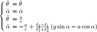
- 1) Find the state equations of the system.
- 2) Let us assume that
 . For which values of ℓ1 and ℓ2 does the pendulum remain vertical, for any horizontal movement of the pendulum? What values does ℓ2 have to take if we let ℓ4 = 1 m and we take r = 6 400 km for the Earth’s radius?
 - 3) Let us assume that, as a result of disturbances, the pendulum starts to oscillate. The period of these oscillations is called the Schuler period. Calculate this period.
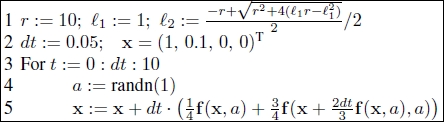
- 4) Simulate the system graphically by taking a Gaussian white noise as the acceleration input. Since the system is conservative, an Euler integration method will not perform well (the pendulum would gain energy). A higher-order integration scheme, such as that of Runge Kutta, should be used. This is given by:
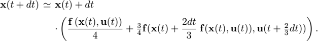
For an easier graphical representation, we will take r = 10 m, ℓ1 = 1 m and g =10 ms−2. Discuss the results.
EXERCISE 1.8.– Brake detector
We will now look at a problem that involves basis changes and rotation matrices. A car is preceded by another car m (which we will assume to be a point). We attach to this car the coordinate system ![]() as represented in Figure 1.12. The coordinate system
as represented in Figure 1.12. The coordinate system ![]() is a ground frame assumed to be fixed.
is a ground frame assumed to be fixed.
This car is equipped with the following sensors:
- – several odometers placed on the rear wheels, allowing us to measure the speed v of the center of the rear axle;
- – a gyro giving the angular speed of the car
 , as well as the angular acceleration
  ;
; - – an accelerometer placed at o1, allowing us to measure the acceleration vector (α, β) of o1 expressed in the coordinate system
 ;
; - – using two radars placed at the front, our car is capable of (indirectly) measuring the coordinates (α1,b1) of the point m in the coordinate system
 as well as the first two derivatives
  and
and  .
.
On the other hand, the car is not equipped with a positioning system (such as a GPS, for example) that would allow it to gain knowledge of ![]() . It does not have a compass for measuring the angle θ. The quantities in play are the following:
. It does not have a compass for measuring the angle θ. The quantities in play are the following:
When a quantity is measured, we assume that its differentials are also measured, but not their primitive. For example, ![]() are considered to be measured since a1, b1 are measured. However,
are considered to be measured since a1, b1 are measured. However, ![]() is measured but θ isn’t. We do not know the state equations of our car. The goal of this problem is finding a condition on the measured variables (and their derivatives) that will allow us to tell whether the point m is braking or not. We understand that such a condition would allow us to build a warning system informing us that the preceding vehicle is braking, even when its rear brake lights are not visible (fog, trailer without brake lights, etc.) or defective.
is measured but θ isn’t. We do not know the state equations of our car. The goal of this problem is finding a condition on the measured variables (and their derivatives) that will allow us to tell whether the point m is braking or not. We understand that such a condition would allow us to build a warning system informing us that the preceding vehicle is braking, even when its rear brake lights are not visible (fog, trailer without brake lights, etc.) or defective.

Figure 1.12. Car trying to detect whether the point m is braking
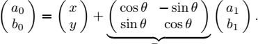
- 1) By expressing the Chasle relation (o0 m = o0o1 + o1 m) in the coordinate system
 , show the basis change formula:

where Rθ is a rotation matrix.
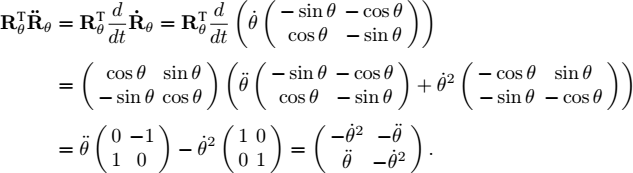
- 2) Show that
 is a skew-symmetric matrix and find its expression.
 - 3) Let u be the speed vector of the point m viewed by a fixed observer. Find an expression
 of the speed vector u expressed in the coordinate system
  . Express
  in function of the measured variables
 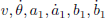 .
. - 4) We will now use the accelerometer of our vehicle, which gives us the acceleration vector (α, β) of o1, expressed in
 . By differentiating
  two times, give the expression of the acceleration
  of m in the coordinate system
  . Deduce from this its expression
  in the coordinate system
  . Give the expression of
  only in function of the measured variables.
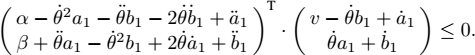
 - 5) Find a condition on the measurements
 which allows us to detect whether the vehicle in front is braking.
EXERCISE 1.9.– Modeling an underwater robot
The robot we will be modeling is the Redermor (greyhound of the sea in the Breton language). A photograph is shown in Figure 1.13. It is an entirely autonomous underwater robot. This robot, developed by GESMA (Groupe d’Etude Sous-Marine de l’Atlantique – Atlantic underwater research group), has a length of 6 m, a diameter of 1 m and a weight of 3,800 kg. It has an efficient propulsion and control system with the aim of finding mines on the seabed.

Figure 1.13. Redermor built by GESMA (Groupe d’Etude Sous-Marine de l’Atlantique –Atlantic underwater research group), on the water surface, still close to the boat it was launched from
Let us build a local coordinate system ![]() over the area traveled by the robot. The point o0 is placed on the surface of the ocean. The vector i0 indicates north, j0 indicates east and k0 is oriented towards the center of the Earth. Let p = (px, py, pz) be the coordinates of the center of the robot expressed in the coordinate system
over the area traveled by the robot. The point o0 is placed on the surface of the ocean. The vector i0 indicates north, j0 indicates east and k0 is oriented towards the center of the Earth. Let p = (px, py, pz) be the coordinates of the center of the robot expressed in the coordinate system ![]() . The state variables of the underwater robot are its position p in the coordinate system
. The state variables of the underwater robot are its position p in the coordinate system ![]() , its tangential v and its three Euler angles φ, θ, ψ. Its inputs are the tangential acceleration
, its tangential v and its three Euler angles φ, θ, ψ. Its inputs are the tangential acceleration ![]() as well as three control surfaces which act respectively on ωx, ωy, ωz. More formally, we have:
as well as three control surfaces which act respectively on ωx, ωy, ωz. More formally, we have:
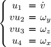
where the factor v preceding u2, u3 indicates that the robot is only able to turn left/right (through u3) or up/down (through u2) when it is advancing. Give the kinematic state model for this system.
EXERCISE 1.10.– 3D robot graphics
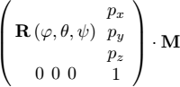
Drawing two- or three-dimensional robots or objects on the screen is widely used for simulation in robotics. The classic method (used by OPENGL) relies on modeling the posture of objects using a series of affine transformations (rotations, translations, homotheties) of the form:
with n = 2 or 3. However, the manipulation of compositions of affine functions is less simple than that of linear applications. The idea of the transformation in homogeneous coordinates is to transform a system of affine equations into a system of linear equations. Notice first of all that an affine equation of the type y = Ax + b can be written as:
We will thus define the homogeneous transformation of a vector as follows:
Thus, an equation of the type
involving the composition of three affine transformations, can be written as:
A pattern is a matrix with two or three rows (depending on whether the object is in the plane or in space) and n columns representing the n vertices of a rigid polygon embodying the object. It is important that the union of all the segments formed by two consecutive points of the pattern forms all the vertices of the polygon that we wish to represent.
1) Let us consider the underwater robot (or AUV, short for Autonomous Underwater Vehicle) whose pattern matrix in homogeneous coordinates is:
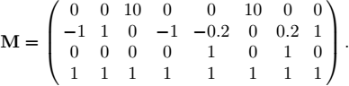
Draw this pattern in perspective view on a piece of paper.
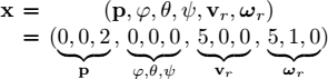
2) The state equations of the robot are the following:
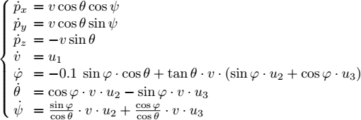
where (φ, θ, ψ) are the three Euler angles. The inputs of the system are the tangential acceleration u1, the pitch u2 and the yaw u3. The state vector is therefore equal to x = (px, py, pz, v, φ, θ, ψ). Give a function capable of drawing the robot in 3D together with its shadow, in the plane x-y. Verify that the drawing is correct by moving the six degrees of freedom of the robot one by one. Obtain a three-dimensional representation such as the one illustrated in Figure 1.14.
3) By using the relation
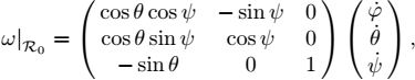
draw the instantaneous rotation vector of the robot.
4) Simulate the robot in various conditions using a Euler method.
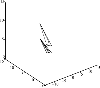
Figure 1.14. 3D representation of the robot together with its shadow in the horizontal plane
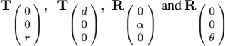
EXERCISE 1.11.– Manipulator robot

Figure 1.15. Parametrization for the direct geometric model of a manipulator robot
A manipulator robot, such as Staubli (represented on Figure 1.15), is composed of several rigid arms. We retrieve the coordinates of the end effector, at the extremity of the robot, using a series of geometric transformations. We can show that a parametrization with four degrees of freedom allows us to represent these transformations. There are several possible parametrizations, each with its own advantages and disadvantages. The most widely used one is probably the Denavit–Hartenberg parametrization. In the case where the articulations are rotational joints (as is the case of the Staubli robot where the joins can turn), the parametrization represented by the figure might prove to be practical since it makes it easier to draw the robot. This transformation is the composition of four elementary transformations: (i) a translation of length r following z; (ii) a translation of length d following x; (iii) a rotation of α around y and (iv) a rotation of θ (the variable activated around z). Using the figure for drawing the arms and the photo for the robot, perform a realistic simulation of the robot’s movement.
EXERCISE 1.12.– Floating wheel
Consider a wheel floating and spinning in the space as shown on Figure 1.16.
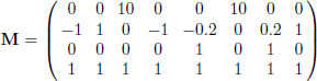
We assume that the wheel is solid, similar to a homogeneous disk of mass m = 1 and radius ρ =1. Its inertia matrix is given by:
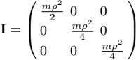
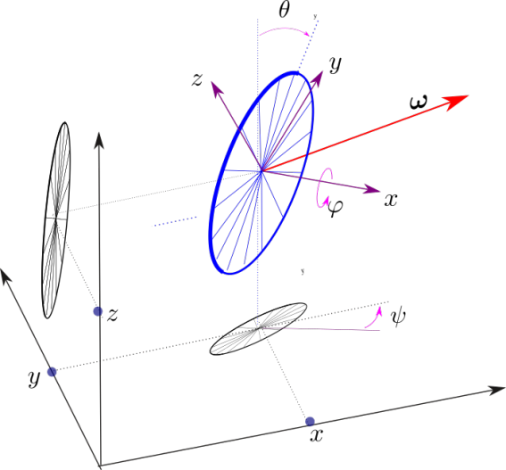
Figure 1.16. Floating wheel. For a color version of this figure, see www.iste.co.uk/jaulin/robotics.zip
- 1) Give the state equations of the wheel. The state variables we choose are (i) the coordinates p = (x, y, z) of the center of the wheel, (ii) the orientation (φ, θ, ψ) of the wheel, (iii) the speed vr of the center of the wheel in the wheel frame, and (iv) the rotation vector ωr expressed in the wheel frame. We thus have a system of order 12.
- 2) The torque-free precession occurs when the angular velocity vector changes its orientation with time. Provide a simulation illustrating the precession.
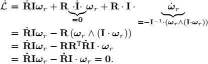
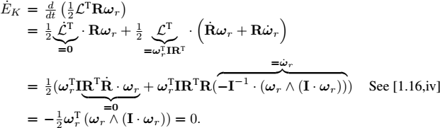
- 3) Show that the angular momentum ℒ = R · I · RT · ω and the kinetic energy
 are both constant. Verify this with a simulation.
 - 4) Using symbolic computation, compute the Jacobian matrix of the evolution function f at point
Give an interpretation.
EXERCISE 1.13.– Schuler oscillations in an inertial unit
Consider the Earth as static, without rotation, with a gravity field directed toward the center and with a magnitude g = 9.81ms−2. An inertial unit is fixed in a robot ![]() at the surface of Earth of radius r. Its position is with p = (r, 0, 0) and its Euler angles rate is (φ, θ, ψ) = (0, 0, 0) as in Figure 1.17. The robot
at the surface of Earth of radius r. Its position is with p = (r, 0, 0) and its Euler angles rate is (φ, θ, ψ) = (0, 0, 0) as in Figure 1.17. The robot ![]() will always be static in the exercise.
will always be static in the exercise.
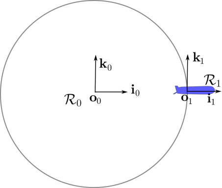
Figure 1.17. The inertial unit inside the robot is static
- 1) Give the values for
 and ωr collected by the inertial unit of
  .
. - 2) We now want to lure the inertial unit by initializing the robot at some other place, say
 , and finding a trajectory so that the unit believes that it is fixed in
  . More precisely, we want to find a motion p(t) = (x(t), y(t), z(t)) for
  so that the inertial unit senses exactly the inputs
  , ωr of
  . For this, we assume that at time t = 0, (φ, θ, ψ) = (0, 0, 0) for
  . For simplicity, we also assume that
  remains in the plane y = 0. Simplify the state equations for
  in our specific case.
 - 3) Provide a simulation of the trajectory of
 , initialized at p(0) = (r, 0, 1)T. Interpret.
 - 4) Linearize the state equation for
 at the state vector corresponding to
  . Compute the eigenvalues and give an interpretation.
 - 5) Assuming that the inertial unit is not perfectly initialized, what can you conclude for the corresponding error propagation?
EXERCISE 1.14.– Lie bracket for control
Consider two vector fields f and g of ℝn corresponding to two state equations ![]() and
and ![]() . We define the Lie bracket between these two vector fields as
. We define the Lie bracket between these two vector fields as
We can check that the set of vector fields equipped with the Lie bracket is a Lie algebra. The proof is not difficult but it is tedious and will not be demanded in this exercise.
1) Consider the linear vector fields f(x) = A · x, g(x) = B · x. Compute [f, g](x).
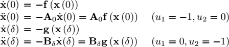
2) Consider the system
We propose to apply the following cyclic sequence:
where δ is an infinitesimal time period δ. This periodic sequence will be denoted by
Show that
3) Which periodic sequence should we take in order to follow the field ν · [f, g]? We will first consider the case ν ≥ 0 and then the case ν ≤ 0.
4) Propose a controller such that the system becomes
where a = (a1, a2, a3) is the new input vector.
5) Consider a Dubins car described by the following state equations:

where u1 is the speed of the car, θ its orientation and (x, y) the coordinates of its center. Using Lie brackets, add a new input to the system, i.e. a new direction of control.
6) Propose a simulation to check the good behavior of your controller. To do this, take δ small enough to be consistent with the second order Taylor approximation but large with respect to the sampling time dt. For instance, we may take ![]() . The initial state vector is taken as x(0) = (0, 0, 1).
. The initial state vector is taken as x(0) = (0, 0, 1).
7) Propose a controller so that the car goes up. Consider the same questions, where the car goes down, right and left, respectively.
EXERCISE 1.15.– Follow the equator
We consider a mobile body moving around a planet, Earth, with a radius ρE rotating along the vertical axis with a rotation rate ![]() .
.
1) Draw Earth rotating with a static body at position p with the following frames (see Figure 1.18):
- i)
 is the Earth-centered inertial frame, fixed with respect to the stars.
 - ii)
 is the Earth frame and turns with the Earth with a rotational speed
  .
. - iii)
 is the navigation frame, ego-centered and pointing towards the sky.
 - iv)
 is the ego-centered frame of the robot.
For the simulation, take ![]() , ρE = 10m.
, ρE = 10m.
2) Provide the kinematic state equations for the body. The state variables are taken as (p, R3, v3), where p is the position of the body in ![]() , R3 is the orientation of the body, and v3 is the speed of the body seen from
, R3 is the orientation of the body, and v3 is the speed of the body seen from ![]() and expressed in
and expressed in ![]() . The inputs are chosen as ω3, the rotation vector of the body and a3, the measured acceleration, both expressed in
. The inputs are chosen as ω3, the rotation vector of the body and a3, the measured acceleration, both expressed in ![]() . Propose a simulation with Earth rotating and the body moving in space with a gravity given by
. Propose a simulation with Earth rotating and the body moving in space with a gravity given by ![]() .
.

Figure 1.18. Earth with the different frames. The origin of the frames have been shifted for more visibility. For a color version of this figure, see www.iste.co.uk/jaulin/robotics.zip
3) The planet is now assumed to be made of water and the body is an underwater robot equipped with actuators (such as propellers) to move inside the water. The gravity is taken as ![]() . The water of the rotating planet drags the robot through friction forces (tangential and rotational). Moreover, the robot, which has the same density as the surrounding fluid, receives an Archimedes upward buoyant force. Propose a dynamical model describing the motion of the robot. The inputs will be the rotational acceleration uω3 and the tangential acceleration ua3 expressed in R3. These accelerations result from the action of the actuators creating forces and torques on the robot. Propose a simulation illustrating all these effects.
. The water of the rotating planet drags the robot through friction forces (tangential and rotational). Moreover, the robot, which has the same density as the surrounding fluid, receives an Archimedes upward buoyant force. Propose a dynamical model describing the motion of the robot. The inputs will be the rotational acceleration uω3 and the tangential acceleration ua3 expressed in R3. These accelerations result from the action of the actuators creating forces and torques on the robot. Propose a simulation illustrating all these effects.
4) The robot behaves like a 3D Dubins-like car model. More precisely, it is equipped with a single propeller which pushes the robot forward without any possibility of controlling the speed. We take ua3 = (1, 0, 0)T. We assume that the robot can chose its rotation vector using rudders, jet pumps or inertial wheels. Find a controller such that the robot goes east along the equator. Validate this with a simulation.
1.6. Corrections
CORRECTION FOR EXERCISE 1.1.– (Properties of the adjoint matrix)
1) The characteristic polynomial of the matrix Ad (ω) is given by:
From this we obtain the eigenvalues {0, ∥ω∥i, −∥ω∥i}. Finally, we have:
and therefore the eigenvector associated with 0 is ω. The matrix Ad (ω) is associated with a speed vector field of a turning coordinate system with ω. Since the axis ω does not move, we will have Ad (ω) · ω = 0.
2) (i) We now show that x ⊥ (ω ∧ x). For this, it is sufficient to prove that xT Ad (ω) x = 0. We have:
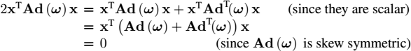
(ii) Since
we get that ω ⊥ (ω ∧ x).
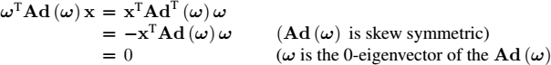
(iii) it is easily shown that:
For this, we need to develop the two expressions above and verify their equality. The positivity of the determinant implies that the trihedron (ω, x, ω ∧ x) is direct.
3) The parallelepiped carried by ω, x and ω ∧ x has a volume of:

However, since ω ∧ x is orthogonal to x and to ω, the volume of the parallelepiped is equal to the surface of its basis ![]() multiplied by its height h = ∥ω ∧ x∥, i.e.:
multiplied by its height h = ∥ω ∧ x∥, i.e.:
By equating the two expressions for v we obtain ![]() .
.
CORRECTION FOR EXERCISE 1.2.– (Jacobi identity)
1) We have

Therefore, for all c
Or equivalently
2) We simply have:
3) We have
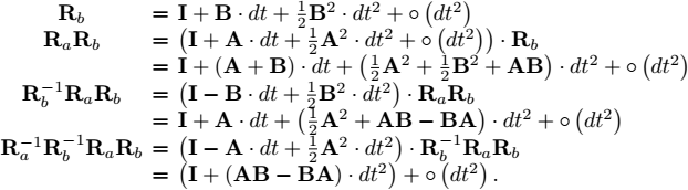
Thus, ![]() corresponds to an infinitesimal rotation following the skew symmetric matrix [A, B] = AB − BA.
corresponds to an infinitesimal rotation following the skew symmetric matrix [A, B] = AB − BA.
As a consequence, if in a space probe, we are able to generate only two rotation motions following A and B using inertial disks, we can also generate a rotation following [A, B] alternating the sequence of infinitesimal rotations with respect to B, A, −B, −A, B, A, −B, −A,…
4) The verification is trivial and we will not give it here. Let us note that this result enables us to deduce that the set of skew-symmetric matrices equipped with addition, bracket and the standard outer product is also a Lie algebra.
CORRECTION FOR EXERCISE 1.3.– (Varignon’s formula)
The position of a point x of the solid body satisfies the state equation:
where ω is parallel to the axis of rotation Δ and ∥ω∥ is the rotation speed of the solid (in rad.s−1). After integrating this linear state equation, we find:
We could also have obtained this formula by applying Rodrigues’ formula studied in exercise 1.4. This property can be interpreted by the fact that Ad (ω) represents a rotation movement, whereas its exponential represents the result of this movement.
CORRECTION FOR EXERCISE 1.4.– (Rodrigues’ formula)
1) It is sufficient to verify that:
2) The solution of the state equation is:
3) At time t the solid body has turned by an angle of ∥ω∥ · t and therefore for t =1, it has turned by ∥ω∥. Therefore, the rotation R of angle ∥ω∥ around ω is given by:
4) The characteristic polynomial of A is ![]() . The eigenvalues of A are 0, i∥ω∥, −i∥ω∥. The eigenvectors associated with the eigenvalue 0 are collinear to ω. This is logical since the points of the axis of rotation have zero speed.
. The eigenvalues of A are 0, i∥ω∥, −i∥ω∥. The eigenvectors associated with the eigenvalue 0 are collinear to ω. This is logical since the points of the axis of rotation have zero speed.
5) The eigenvalues of R are obtained using the eigenvalue correspondence theorem and are therefore equal to e0, ei∥ω∥,e−i∥ω∥.
6) The expression of a rotation around the vector ω = (1, 0, 0) of angle α is:
7) Rodrigues’ formula tells us that the orientation matrix around the vector ω of angle φ = ∥ω∥ is given by:
CORRECTION FOR EXERCISE 1.5.– (Geometric approach to Rodrigues’ formula)
1) We have:
Whence Rodrigues’ formula:
2) We have:
Therefore:
Rodrigues’ formula can therefore also be written as:
The operator can be represented by the following rotation matrix:
or, in a developed form:
3) We have
Moreover
Thus
4) The trajectory has the form R(t) = exp (tA) · Ra and we have to find A which is skew-symmetric (so that exp (tA) is a rotation matrix). For t = 0, we have R(0) = Ra and for t = 1, we want R(1) = Rb. We thus have to solve Rb = exp (A) · Ra or equivalently ![]() , with A skew-symmetric. We may write
, with A skew-symmetric. We may write ![]() but the logarithm of a matrix is not unique. In this exercise, it is assumed that all matrices are of dimension 3 × 3. To find an interpolation trajectory matrix R(t) between Ra and Rb, we take the results of the previous question and we perform the following
but the logarithm of a matrix is not unique. In this exercise, it is assumed that all matrices are of dimension 3 × 3. To find an interpolation trajectory matrix R(t) between Ra and Rb, we take the results of the previous question and we perform the following

Then, we get R(t) = exp (tA) · Ra. We clearly see here that finding A such that ![]() is not a unique solution. For instance, we could have taken A = (φ + 2kπ) n∧, with k ≠ 0, but several turns are now needed to go from Ra to Rb.
is not a unique solution. For instance, we could have taken A = (φ + 2kπ) n∧, with k ≠ 0, but several turns are now needed to go from Ra to Rb.
5) Let us recall that the Maclaurin series development of the sine and cosine functions is written as
Let H = Ad (n). Since n is an eigenvector of H associated with the zero eigenvalue, we have H (n · nT) = 0. Moreover
Therefore
Thus, Rodrigues’ formula is written as

Or equivalently
CORRECTION FOR EXERCISE 1.6.– (Quaternions)
1) We have:
| · | 1 | i | j | k |
| 1 | 1 | i | j | k |
| i | i | −1 | k | −j |
| j | j | −k | −1 | i |
| k | k | j | −i | −1 |
Note that the multiplication is not commutative.
2) We have

3) Both quaternions ![]() , and
, and ![]() correspond to the same rotation. Now,
correspond to the same rotation. Now,
4) We have:
5) (i). Since the rotations are simple, the first method is to get the result directly by hand moving a simple object for instance. We obtain a rotation with respect to (0, 1, 0) with an angle ![]() .
.
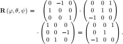
(ii) We build the rotation Euler matrix R associated to ![]() . We get
. We get
Then, we take one normalized eigenvector v of R associated with the eigenvalue λ =1: v = (0, 1, 0)T. The rotation R can be obtained as a rotation of an angle α around v. To compute α, we apply the formula [1.9]
where the sign chosen to have eα·v∧ = R. We get ![]() .
.
(iii) We now use the quaternion method. We get
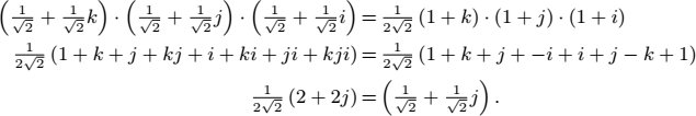
With all approaches, we obtain a rotation with an angle ![]() around the vector v = (0, 1, 0).
around the vector v = (0, 1, 0).
CORRECTION FOR EXERCISE 1.7.– (Schuler pendulum)
1) The state vector is ![]() . In order to have a horizontal movement, we need a horizontal force f. Following the fundamental principle of dynamics, we have:
. In order to have a horizontal movement, we need a horizontal force f. Following the fundamental principle of dynamics, we have:
with ![]() and f = 2ma. Since
and f = 2ma. Since ![]() , the state equations of the system are written as:
, the state equations of the system are written as:
2) The pendulum remains vertical if, for α = 0, we have ![]() . Thus
. Thus
or equivalently:
We must therefore satisfy the equation ![]() . Solving it gives:
. Solving it gives:
For ℓ1 = 1, we obtain:
3) The equation describing the oscillations is:
For a = 0, we have:
which is the equation of a pendulum of length ℓ = r. By linearizing this equation, we obtain the characteristic polynomial ![]() and therefore the pulse
and therefore the pulse ![]() . The Schuler period is therefore equal to:
. The Schuler period is therefore equal to:
4) The program is the following:
Note that for an initialization ![]() , the pendulum always points towards the center of the Earth. Otherwise, it oscillates and conserves this oscillation at the Schuler frequency. This oscillation can be observed in modern inertial units and there are methods for compensating for it using information gathered by the other inertial sensors.
, the pendulum always points towards the center of the Earth. Otherwise, it oscillates and conserves this oscillation at the Schuler frequency. This oscillation can be observed in modern inertial units and there are methods for compensating for it using information gathered by the other inertial sensors.
CORRECTION FOR EXERCISE 1.8.– (Brake detector)
1) We have:
Let us express this relation in the coordinate system ![]() :
:
which leads to:
2) We have:
3) in the coordinate system ![]() this vector u is expressed by:
this vector u is expressed by:
Therefore:

4) We have:

Therefore:

However:
We get
5) The vehicle in front of us is braking if
i.e. if
CORRECTION FOR EXERCISE 1.9.– (Modeling an underwater robot)
The derivative of the position vector is obtained by noticing that:

since i1 corresponds to the first column of matrix [1.9]. Finally, by taking into account equations [1.12], we can write the state equations for our submarine:

Here we have a kinematic model (i.e. it does not involve forces or torques). There are no parameters and the model can therefore be considered correct if the underwater robot is solid (that is, it cannot be contorted), and if its trajectory is tangent to the axis of the robot. Such a model allows us to use nonlinear control methods such as feedback linearization which will be discussed in Chapter 2. These methods are indeed less robust with respect to a model error, but are formidably efficient if an accurate model for our system is known.
CORRECTION FOR EXERCISE 1.10.– (3D robot graphics)
2) To draw the robot at state x = (px, py, pz, v, φ, θ, ψ), we build the pattern matrix
 and we compute the transformed pattern matrix (to be painted)
3) The simulation could be done by using Euler’s integration method as shown by Figure 1.19 with the initial vector
and the control u = (0, 0, 0.2)T. This simulation will be picked up in exercise 2.4 for performing the control of the trajectory of the robot.

Figure 1.19. Simulation of the underwater robot. For a color version of this figure, see www.iste.co.uk/jaulin/robotics.zip
CORRECTION FOR EXERCISE 1.11.– (Manipulator robot)
One must draw the arms one after the other. For this, we have to build the translation by a vector v and the rotation around ω with an angle ∥ω∥. They are represented by the two matrices

In this exercise, we need a translation of length r following the z-axis, a translation of length d following x, a rotation of α around y and a rotation of θ. They are respectively given by the 4 × 4 matrices
The seven arms of the robot in a configuration q (whose components are the coordinates of the articulations) can be drawn as follows:
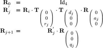
Each arm is drawn using the pair of two homogeneous matrices ![]() , for j ∈ {1,…, 7}. Figure 1.20 corresponds to a simulation for a robot with the following parameter vectors:
, for j ∈ {1,…, 7}. Figure 1.20 corresponds to a simulation for a robot with the following parameter vectors:

CORRECTION FOR EXERCISE 1.12.– (Floating wheel)
1) Considering the Euler’s rotation equation
where the torque τr = 0, and the fact that we have no acceleration of our wheel, from [1.12] we get

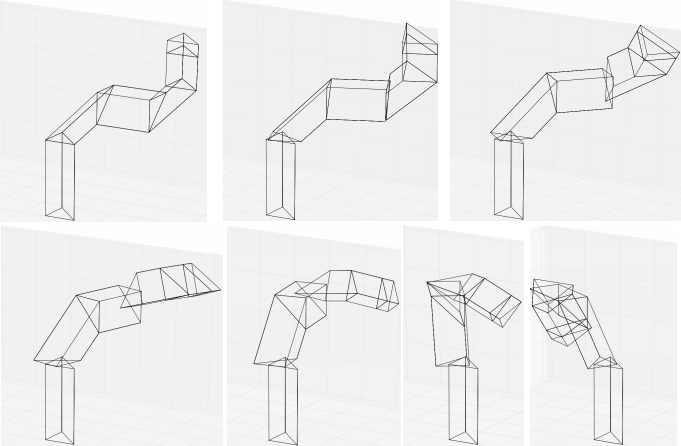
Figure 1.20. Simulation the manipulator robot
2) For the simulation, we take
and we get the result depicted in Figure 1.12. The wheel translates with respect to px. We see from the shadow (black) that the rotation axis oscillates. This corresponds to the precession.

Figure 1.21. Motion of the wheel with a torque-free precession. For a color version of this figure, see www.iste.co.uk/jaulin/robotics.zip
3) We have ℒ = RIRTω = RIωr. Therefore
Moreover
4) We write the following PYTHON code using the SYMPY library:
from sympy import *x = MatrixSymbol(’x’, 12, 1)wx, wy, wz, rho, m, s=symbols(“wx wy wz rho m s”)phi, theta, psi=x[3:6]vr=Matrix(x[6:9])wrx, wry, wrz=x[9:12]wr=Matrix(x[9:12])ci, si, cj, sj, ck, sk=cos(phi), sin(phi), cos(theta), sin(theta),cos(psi),sin(psi)Ri = Matrix([[1, 0, 0], [0, ci, -si], [0, si, ci]])Rj = Matrix([[cj, 0, sj], [0, 1, 0], [-sj, 0, cj]])Rk = Matrix([[ck, -sk, 0], [sk, ck, 0], [0, 0, 1]])E= Rk*Rj*Ridp=E*vrda= Matrix([[1, si*sj/cj, ci*sj/cj], [0, ci, -si],[0, si/cj, ci/cj]])*wrA=Matrix([[0, -wrz, wry], [wrz, 0, -wrx], [-wry, wrx, 0]])dvr=-A*vrI=(m/2)*rho**2*Matrix([[1, 0, 0], [0, 1/2, 0], [0, 0, 1/2]])dwr=-(I**-1)*(A*I*wr)f=Matrix((dp, da, dvr, dwr))J=f.jacobian(x)x0=Matrix([[0], [0], [0], [0], [0], [0], [0], [0], [0], [wx], [wy], [wz]])J=J.subs(x, x0)
The matrix J at point x0 is written in Figure 1.23.
The yellow blocks with zeros can be understood by the graph of Figure 1.23. An arc represents a differential delay. For instance, the arc between the node vr and p means that ![]() depends algebraically on vr.
depends algebraically on vr.
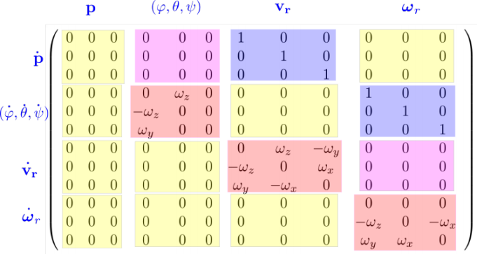
Figure 1.22. Jacobian matrix of the evolution function at point xo. For a color version of this figure, see www.iste.co.uk/jaulin/robotics.zip

Figure 1.23. Graph of the differential delays for the floating wheel. For a color version of this figure, see www.iste.co.uk/jaulin/robotics.zip
The matrix J is block triangular and we can easily compute the characteristic polynomial. It is given by
The term ![]() is consistent with the fact when no precession exists, the wheel spins around ωr at a pulsation ∥ωr∥. The terms
is consistent with the fact when no precession exists, the wheel spins around ωr at a pulsation ∥ωr∥. The terms ![]() and
and ![]() correspond to the precession.
correspond to the precession.
If the wheel is not perfectly solid, internal frictions will tend to dampen the precession, and the rotation axis will align itself with one eigenvector of I. This vector can either be one vector of the wheel plane, or the axis of the wheel (orthogonal to the wheel plane).
CORRECTION FOR EXERCISE 1.13.– (Schuler oscillations in an inertial unit)
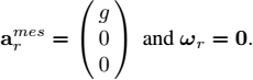
1) Since the Earth is static, we have
2) All Euler angles of ![]() are constant (as for
are constant (as for ![]() ) and equal to zero. They do not appear as state variables anymore. The Euler matrix R (φ, θ, ψ) is equal to the identity. The state equations of
) and equal to zero. They do not appear as state variables anymore. The Euler matrix R (φ, θ, ψ) is equal to the identity. The state equations of ![]() become
become

They can be rewritten as follows:
3) We get the trajectory represented in Figure 1.24. We observe some oscillations known as the Schuler oscillations.
4) Around z = 0, x = r, we get
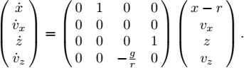
The eigenvalues are ![]() . Some oscillations exist and this system is unstable due to the fact that we have two roots in 0.
. Some oscillations exist and this system is unstable due to the fact that we have two roots in 0.
5) In practice, the inertial unit is not perfectly initialized, and thus it finds a trajectory similar to that of ![]() whereas it is fixed for
whereas it is fixed for ![]() . Since the error is small, the linear approximation is realistic. The integration method inside the inertial unit returns some unwanted oscillations corresponding to a solution which is not the actual one, as illustrated by Figure 1.25. These oscillations correspond to a period
. Since the error is small, the linear approximation is realistic. The integration method inside the inertial unit returns some unwanted oscillations corresponding to a solution which is not the actual one, as illustrated by Figure 1.25. These oscillations correspond to a period ![]() , named the Schuler period. For many applications (such as when we are in an aircraft), we know that such oscillations are dummies and we may improve the integration method in order to damp these Schuler oscillations.
, named the Schuler period. For many applications (such as when we are in an aircraft), we know that such oscillations are dummies and we may improve the integration method in order to damp these Schuler oscillations.

Figure 1.24. The robot  with the trajectory painted blue and the robot
  fixed in o1 both undergo the same rotation rate and the same acceleration
CORRECTION FOR EXERCISE 1.14.– (Lie bracket for control)
1) We have

2) Without loss of generality, the proof will be given for t = 0. We shall use the following notations
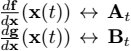
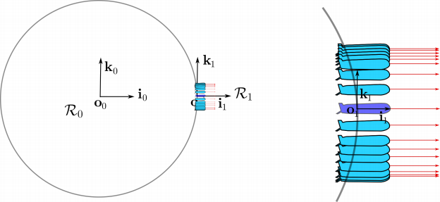
Figure 1.25. Fake periodic trajectory returned by the inertial unit which feels the same as if it were static as for  . The corresponding measured acceleration
  is painted red. The right subpicture corresponds to a zoom around
  . For a color version of this figure, see www.iste.co.uk/jaulin/robotics.zip
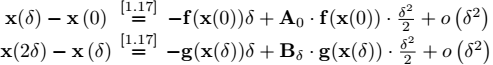
For a given t, and a small δ we have
with
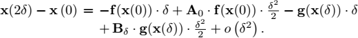
Thus
We get
The sum yields
Now,
(i) ![]()
(ii) Bδ = B0 + o(1)
Therefore

The same reasoning yields

This result could be obtained directly from [1.19] by rewriting: δ → −δ, f → −g, g → −f, A0 → −B0, B0 → −A0. Thus
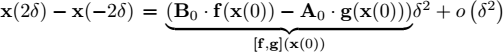
The consequence is that, using the periodic sequence, we are now able to move with respect to the direction [f, g].
3) We have shown that within a time period of 4δ we moved in the direction [f, g] by [f, g]δ2. This means that we follow the field ![]() which is infinitesimal. Multiplying the cyclic sequence by the scalar α ∈ ℝ amounts to multiplying both f, g by α. The field thus becomes
which is infinitesimal. Multiplying the cyclic sequence by the scalar α ∈ ℝ amounts to multiplying both f, g by α. The field thus becomes ![]() . If we want the field ν · [f, g], we have to take multiply the sequence by
. If we want the field ν · [f, g], we have to take multiply the sequence by ![]() . If ν is negative, we have to change the orientation of the sequence. The cyclic sequence is thus
. If ν is negative, we have to change the orientation of the sequence. The cyclic sequence is thus
where ε = sign(ν) changes the orientation of the sequence (clockwise for ε = 1, counterclockwise for ε = −1).
4) If we want to follow the field a1f + a2g + a3[f, g], we have to take the sequence
with ![]() and ε = sign(v).
and ε = sign(v).
5) If we set x = (x, y, θ) we have
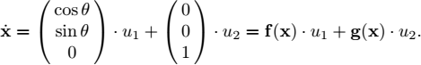
We have
We can now move the car laterally.
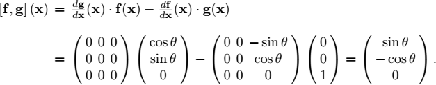
6) if we apply the cyclic sequence as a controller, we get
We made 4 simulations for a = (0.1, 0, 0), a = (0, 0, 0.1), a = (−0.1, 0, 0), a = (0, 0, −0.1). We took for initial vector x(0) = (0, 0, 1), t ∈ [0, 10] and dt = 0.01. We obtained the results depicted by Figure 1.26. We observe that after each simulation, the distance to the origin is 0.1 × 10 = 1 approximately which is consistent with the fact that f (x) and [f, g] have a norm equal to 1. We did not show the simulation for a = (0, ±0.1, 0) since there is no displacement: the car turns on itself.
7) We have
We take a = ![]() , where
, where ![]() .
.
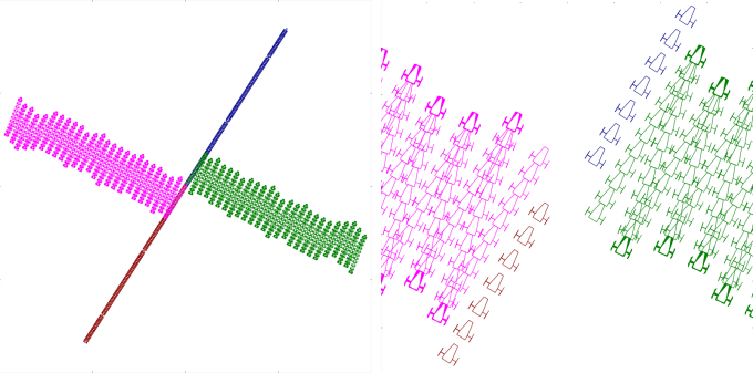
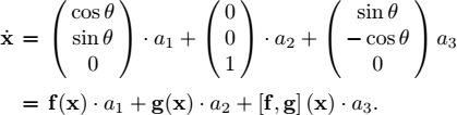
Figure 1.26. Left: simulation of the controller based on the Lie bracket technique. The frame box is [−1, 1] × [−1, 1]. Right: the same picture, but with a frame box equal to [−0.2, 0.2] × [−0.2, 0.2]. To avoid superposition in the picture, the size of the car has been reduced by 1/1000. The length of the forward/backward subpaths corresponds to 10cm approximately. For a color version of this figure, see www.iste.co.uk/jaulin/robotics.zip
For sequentially desired directions: ![]() . We get the results shown in Figure 1.27.
. We get the results shown in Figure 1.27.
CORRECTION FOR EXERCISE 1.15.– (Follow the equator)
1) The rotation matrices to go from one frame to another are ![]() . We have
. We have
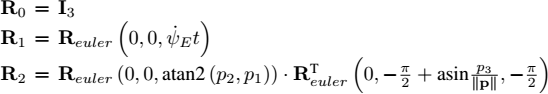
2) The kinematic equations, taken from [1.13], are:
On the simulation (see Figure 1.28), we observe that the trajectory corresponds to an ellipse which is consistent with the behavior of a satellite. The rotation of the body is due to the initial conditions.
Figure 1.27. Left: The car goes from 0 toward all cardinal directions. The frame box is [−1, 1] × [−1, 1]. Right: the same picture, but with a frame box equal to [−0.2, 0.2] × [−0.2, 0.2]. For a color version of this figure, see www.iste.co.uk/jaulin/robotics.zip
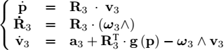
3) The dynamic model is composed of the kinematic model, to which we add the following state equation to generate the inputs a3, ω3 (see Figure 1.29):

This dynamic (left) block has ω3 among the state variables.
Let us explain the first equation:
The friction term tells us that if we have no actuators, the robot will stop its rotation with respect to the water and thus converge on a rotation equation which is that of the Earth. To this friction, we should add the rotation coming from rudders or propellers.
The second equation is composed of three terms


Figure 1.28. The robot moves like a satellite around the Earth. For a color version of this figure, see www.iste.co.uk/jaulin/robotics.zip
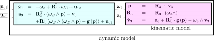
Figure 1.29. Dynamic model
- (i) An acceleration exists due to the friction. As a first approximation, we may assume that the acceleration is proportional to the speed difference between the robot and the fluid. Since the speed of the fluid is vf = ωE ∧ p, we get an acceleration due to the friction that may be approximated in the
 frame by
 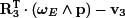 .
. - (ii) The acceleration of the fluid at p is

If the robot is static with respect to the fluid and has the same density as the fluid, it will have the acceleration
 resulting from the Archimedes force. Now, due to the gravity, it will measure the acceleration
 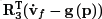 in the
  frame.
 - (iii) The acceleration ua3 coming from the propellers are expressed in the robot frame
 .
.
4) To control the direction of the robot, we consider a pose field approach, i.e. we associate with each point p a pose (represented by a rotation matrix R4) that the robot tries to satisfy. For instance if we want to follow the equator from west to east, we choose as a pose field
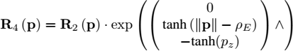
Then, we choose the rotation vector for the control to make R3 like R4 (p). We get (see equation 1.6):
where ![]() and
and ![]() . The corresponding simulation is depicted in Figure 1.30.
. The corresponding simulation is depicted in Figure 1.30.

Figure 1.30. The robot follows the equator toward the east. For a color version of this figure, see www.iste.co.uk/jaulin/robotics.zip